This section just scratches the surface, there are many more commonly used filters. To go further, it would be helpful to look at the following.

• the state variable filter
• the biquad filter
• Robert Bristow-Johnson’s biquad filter cookbook
• IIR and FIR filters
• example filter code on musicdsp.org

If you want to go beyond using filters in your code, you will need to study the signal processing mathematics. It isn’t easy, but now that you are using digital filters in your code, you should have the motivation to dive in.

• One of many online courses in DSP
• Julius O. Smith’s excellent “INTRODUCTION TO DIGITAL FILTERS 
  WITH AUDIO APPLICATIONS”
• UCSD’s MUS270A (occasionally undergrads are given permission to enroll)

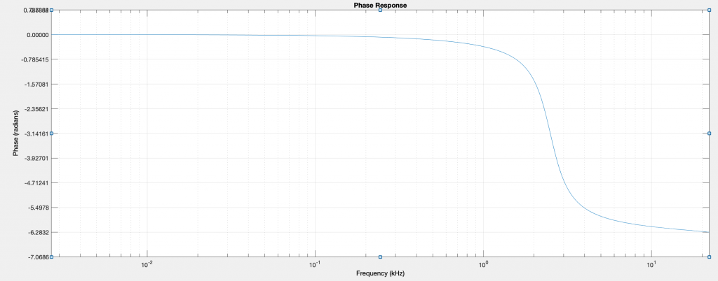
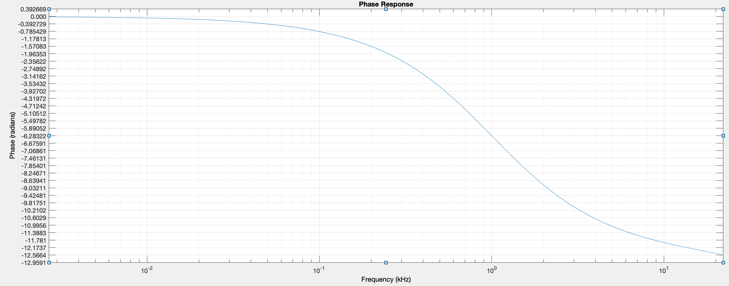
As in the phase shifter, bandreject and bandpass filters can be simply constructed from a second order allpass filter, taking advantage of the phase inversion (-π) at the frequency of the allpass. The input signal will be out of phase with the allpass output at this frequency. Furthermore, the input signal is in phase with the allpass output at frequencies near 0, as well as near the nyquist. Here is the allpass phase response again.

Implementation

Because of this, a band reject filter can be obtained by adding the output of the allpass to the input signal and multiplying the sum by 1/2. This will cancel the signal at the -π frequency and pass it at 0 and nyquist. Note that at the -π/2 (and -3π/2) frequency the sum of a the input (0 phase) and allpass output (-π/2 phase) will be the hypotenuse of the two magnitudes as they are 90 degree apart. The hypotenuse is \sqrt{(1.0^2 + 1.0^2)} = 1.4142135... This sum will be multiplied by 1/2 as well, giving 0.707106… or -3.0103… dB at the bandwidth frequencies.

It follows that band pass filter can be obtained by subtracting the output of the allpass from the input signal and multiplying the sum by 1/2. We can combine these by multiplying the allpass output by a gain factor that varies from -1.0 to 1.0. This will give a filter that can go from bandpass to bandreject smoothly. Here is the C implementation, a simple modification of the second order allpass code.

#define SAMPLERATE 44100.0
#define PI 3.141592653589793
double x0 = 0.0; // input
double x1 = 0.0; // delayed input
double x2 = 0.0; // delayed input
double y0 = 0.0; // allpass output
double y1 = 0.0; // delayed output
double y2 = 0.0; // delayed output

sobpo(float *input, float *output, long samples, float cutoff, float bw) 
{   
    double d = -cos(2.0 * PI * (f/SAMPLERATE));
    double tf = tan(PI * (bw/SAMPLERATE)); // tangent bandwidth   
    double c = (tf - 1.0)/(tf + 1.0); // coefficient     
    for(int i = 0; i < samples; i++) 
    {  
        x0 = *(input+i);   
        y0 = -c*x0 + (d - d*c)*x1 + x2 - (d - d*c) * y1 + c*y2;
        // move samples in delay for next sample
        x2 = x1;
        x1 = x0;
        y2 = y1;
        y1 = y0;
        *(output+i) = (x0 + y0 * factor) * 0.5;
    }
}

Introduction

In the section on phase shifters, 2 first order allpass filters are cascaded to obtain a phase shift of -π in the middle of the frequency range. The -π phase shift makes it possible to implement a band reject filter by adding the input to the phase shifted allpass output or a band pass by subtracting the allpass output from the input.

There are many ways to formulate a second order allpass, but in this section we will be using a filter developed by professor fred harris at SDSU for an efficient parametric equalizer used in an early hybrid guitar amp.

y[n] = -c(x[n]) + (d - dc)x[n-1] + x[n-2] - (d - dc)(y[n-1]) + c(y[n-2])

Above is the difference equation for this allpass. The coefficients are c and d. The input parameters used are frequency and bandwidth. Frequency is the -π phase shift point and bandwidth is the frequency distance between the -π/2 and -3π/2 points.

The coefficients are calculated from frequency (f) and bandwidth (bw) by:

\begin{aligned}& d = -cos\bigg(2\pi \frac{f}{sr} \bigg) \\ & tf = tan\bigg(\pi \frac{bw}{sr} \bigg) \\ & c = \frac{tf-1}{tf+1} \end{aligned}

Notice the d is completely dependent on f and c is completely dependent on bw. The decoupling of coefficients will allow easy optimization of this filter.

The plot above shows that this filter reaches -π/2 at 2000Hz, -π at 2500Hz and -3π/2 at 3000Hz. The C implementation is straightforward and can be derived directly from the difference equation above.

#define SAMPLERATE 44100.0
#define PI 3.141592653589793
double x0 = 0.0; // input
double x1 = 0.0; // delayed input
double x2 = 0.0; // delayed input
double y1 = 0.0; // delayed output
double y2 = 0.0; // delayed output

soap(float *input, float *output, long samples, float cutoff, float bw) 
{   
    double d = -cos(2.0 * PI * (cutoff/SAMPLERATE));
    double tf = tan(PI * (bw/SAMPLERATE)); // tangent bandwidth   
    double c = (tf - 1.0)/(tf + 1.0); // coefficient     
    for(int i = 0; i < samples; i++) 
    {  
        x0 = *(input+i);   
        *(output+i) = -c*x0 + (d - d*c)*x1 + x2 - (d - d*c)y1 + c*y2;
        // move samples in delay for next sample
        x2 = x1;
        x1 = x0;
        y2 = y1;
        y1 = *(output+i);
    }
}

The slope of a one pole filter is -6 dB per octave. A steeper slope can be achieved by connecting multiple one pole filters in series, and giving all of them the same frequency coefficient. It was Robert Moog who developed this technique for synthesis, using four low pass filters in series to make his voicing filter for the Moog 904A filter module in 1966. This filter arrangement (aka ladder filter) has been used in all subsequent Moog synthesizers, as well as most other analog and virtual analog synthesizers.

Moog’s filter has another characteristic that makes it especially flexible. It has a regeneration control (later emphasis) which transforms the low pass filter into a resonant band pass filter, and then a sine oscillator when regeneration is fully on.

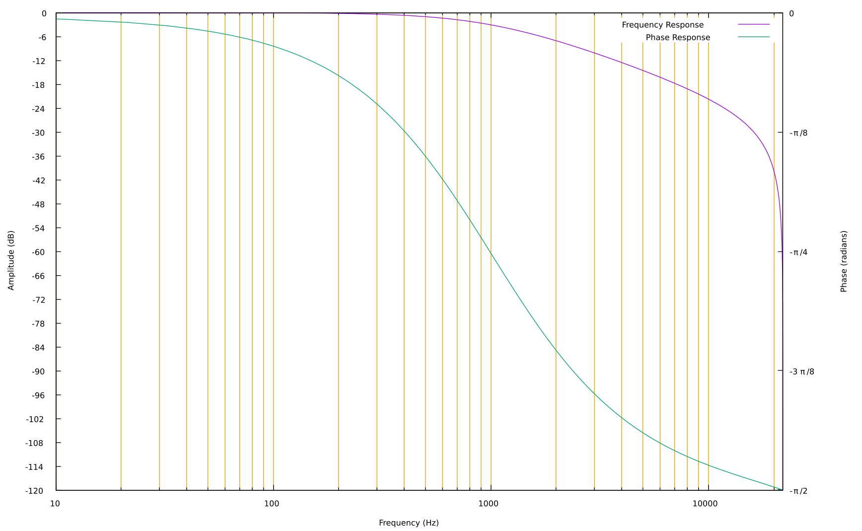
This regeneration control is a negative feedback control, mixing the inverted filter output back into the input. As the control is increased, the low frequencies passing through the filter are reduced, and the signal around the filter frequency is increased. To understand why this happens, consider the frequency and phase response of the low pass filter at 1000Hz.

At 1000Hz, the phase shift is -π/4 and the gain is -3dB. When 4 of these filters are in series, the total phase shift at 1000Hz is -π and the gain is -12dB. A phase shift of -π is a signal inversion at this frequency. If the inverted signal at 1000Hz is inverted again, it will be in phase with the input. By mixing it with the input, the signal at 1000Hz is reinforced.

Below 1000Hz, phase shift moves toward 0. The filtered signal below 1000Hz becomes more in phase with the input signal. By inverting it and mixing back into the input, the sound below 1000Hz will be reduced.

Finally, as regeneration increases, feedback in the filter increases. The sound becomes more resonant – the filter “rings”. In short, by reinforcing the signal at the filter frequency, reducing the signal below the filter frequency, and increasing the filter feedback; this filter moves from being a low-pass filter to a resonant low-pass to a band-pass filter and finally a sine wave oscillator. This is what makes Robert Moog’s design so clever and useful.

Implementation

The C implementation is almost as simple as the description above. The only addition is a saturation section after the negative feedback is added to the input. One could also add saturation after every filter section to emulate the natural saturation in the original transistors. One note: because of the delay in the feedback loop, this implementation of the Moog ladder filter will get slightly out of tune at higher frequencies. There has been some good research in eliminating this feedback delay error. If you want to dig deeper, read Vadim Zavalishin’s The Art of VA Filter Design.

double out1a, out1b, out1c, out1d; // keep track of the last output

ladderFilter(float *input, float *output, long samples, float cutoff, float regeneration) 
{
    double c = exp(-6.283185307179586 * cutoff/samplingRate);

    for(int i = 0; i < samples; i++) 
    {
        float in = *(input+i) - (out1d * regeneration);
        in = 0.636619772367581 * atan(in); // constant is 2/π
        out1a = in * (1 - c) + out1a * c;
        out1b = out1a * (1 - c) + out1b * c;
        out1c = out1b * (1 - c) + out1c * c;
        out1d = out1c * (1 - c) + out1d * c;
        *(output+i) = out1d; 
  }
}

An analog phase shifter (or phaser) is one or more notch (band reject) filters modulated by a slow triangle or sine wave. It’s a fairly common effect, often used on guitar (Something About Us by Daft Punk) or keyboard (Are You All the Things by Bill Evans). The main character of the phase shifter is that of a quickly changing timbre, much like the sound of a Leslie rotating speaker. As it uses a moving notch filter, only a few of the harmonics are affected at any moment. Popular phasers include the MXR Phase 90, the Mu-Tron Bi-Phase, and the Electro Harmonix Small Stone.

Phase shifters are made by using a series of cascaded allpass filters, with the output of the last filter mixed with the input signal. The highest frequency should be shifted by a multiple of 2π and the lowest shifted by 0 in this group of allpass filters, so that the input and output signals are in phase at the top and bottom of the spectrum, and reinforce when mixed together.

Implementation

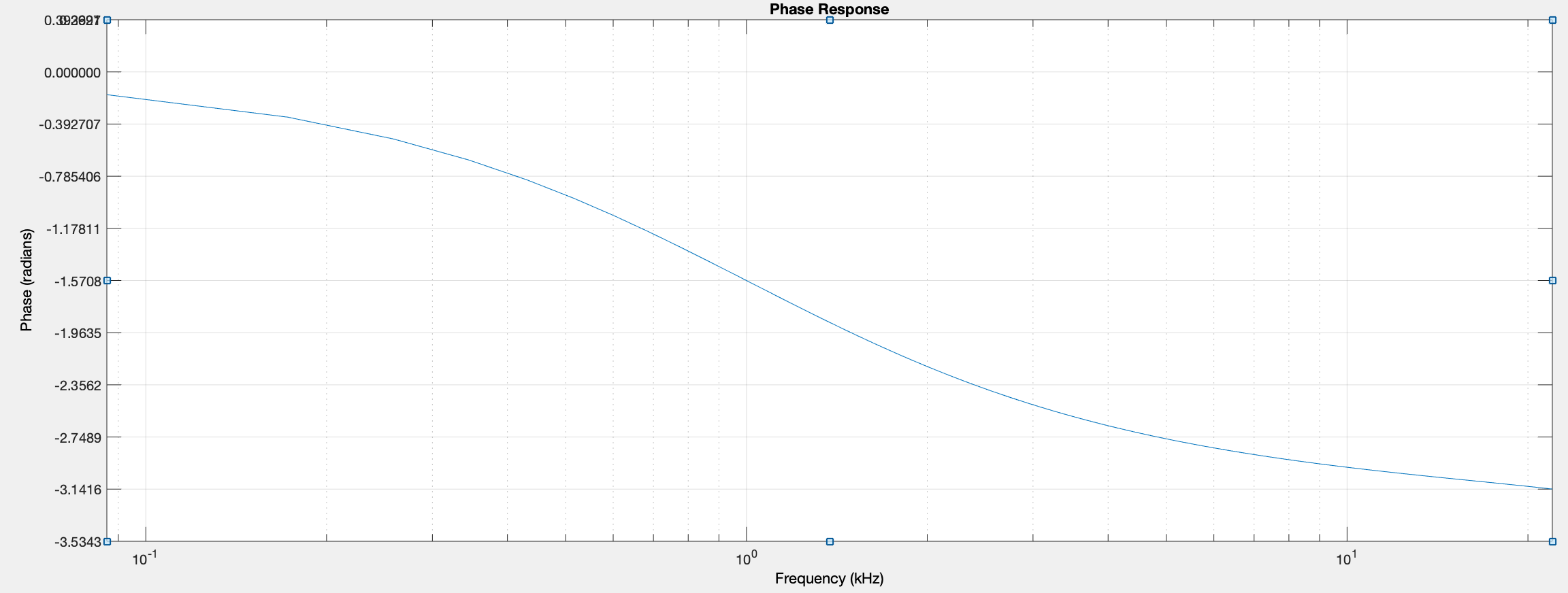
The first order allpass filter introduced earlier can be used for the cascaded filters in a phase shifter. As the first order allpass filter has a phase shift of π at nyquist, 2 of these filters are needed to obtain a phase shift of 2π.

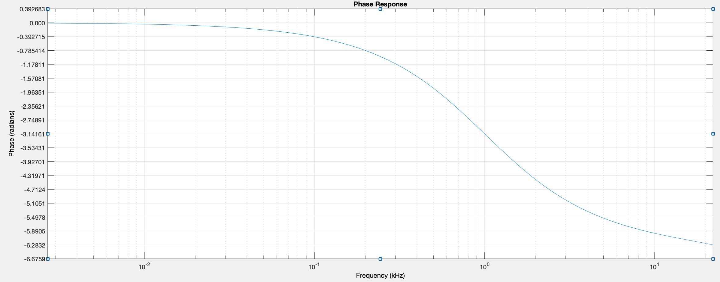
All of the filters in the cascade will have their frequency modulated by the same oscillator. This will move a -π (180) phase shift point up and down through the spectrum. When mixed with the input signal, the -π shift point will create the notch.

If more filters are cascaded, more notches will be created. Sounds at 0, -2π, -4π, -6π, etc. will be reinforced, and sounds at -π, -3π, -5π, etc. will be cancelled. The extra notches will create a deeper, more obviously effected sound, as more harmonics will be removed by the notches. Also important: the multiple notches are no longer harmonically related, and so the phase shifter will not act like a resonant comb filter.

To put this together in C, a slow sine wave is needed. This will modulate the frequency of 4 cascaded first order allpass filters. The output of the last allpass filter will be mixed with the input signal.

// the samplerate in Hz
float sampleRate = 44100;
// the frequency of phase modulation - once every 2 seconds
float frequency = 0.5;
// initial phase
float phase = 0.0;
// x1 and y1 for each allpass stage
double x1a, x1b, x1c, x1d;
double y1a, y1b, y1c, y1d;

void Phaser(float *input, float *output, float frequency, long samples)
{
    long sample;
    float apfreq, tf, c;
    // calculate for each sample in a block
    for(sample = 0; sample < samples; sample++)
    {
        // get the phase increment for this sample
        phaseIncrement = frequency/sampleRate;

        // calculate the allpass frequency (200 to 5000) 
        apfreq = (sin(phase * 6.283185307179586) + 1.0) * 2400.0 + 200;
        // calculate the allpass coefficient
        tf = tan(3.141592653589793 * apfreq/sampleRate);
        c = (tf - 1.0)/(tf + 1.0);

        // compute the 4 allpass filters, and save the previous input
        float x0a = *(input+i);            
        y1a = (c*x0a) + x1a - (c * y1a);
        x1a = x0a;
        y1b = (c*y1a) + x1b - (c * y1b);
        x1b = y1a;
        y1c = (c*y1b) + x1c - (c * y1c);
        x1c = y1b;
        y1d = (c*y1c) + x1d - (c * y1d);
        x1d = y1c;

        // calculate the output for this sample
        *(output+sample) = *(input+sample) + y1d; 

        // increment the phase
        phase = phase + phaseIncrement;
        if(phase >= 1.0)
            phase = phase - 1.0;
    }
}

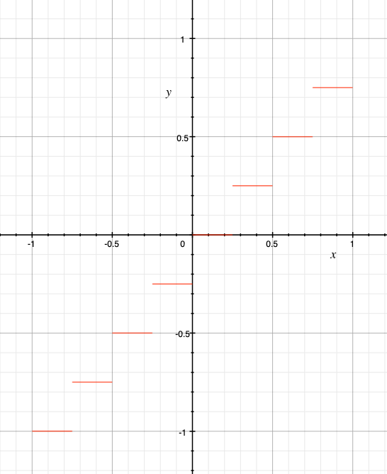
Decimation is a type of waveshaping that reduces the resolution of the input signal by eliminating the lower bits in the integer representation of the sample. For example, lets take a sample of value 0.5337 (within the typical range of 1.0 to -1.0) to 3 bit resolution. With 3 bits, we only have 8 values from -1.0 to 1.0: -1.0. -0.75, -0.5, -0.25, 0.0, 0.25, 0.5, 0.75. The value 0.5337 becomes 0.5 (as do all values between 0.5 and 0.75). This reduction in resolution will create noise which is not related to the amplitude of the signal. The less bits used, the great the decimation noise. If we consider 3-bit decimation a transfer function, it would look like this:

Using a transfer function like the above is one method of decimation. However, as with other types of waveshaping, it is more efficient to compute decimation directly, using the equation which would create the transfer function.

Implementation

The following equation could be used to decimate a floating point signal.

y[n] = \lfloor(x[n] * 2^{(bits - 1)})\rfloor/(bits-1)

Below are two C implementations of decimation to 3 bits. First using multiplication and division, and the second using logical bit operations. The logical operations are probably much less CPU intensive.

// decimation to 3 bits using multiplication and division

factor = pow(2.0, bits - 1.0);
output = floor(input * factor)/factor;

// decimation to 3 bits using logical operations

// convert to 16-bit sample
input16 = (int)(input * 32768);
// zero out all but the top 3 bits using bitwise and
// binary literals only allowed in gcc, in hex use 0xe000
output16 = input16 & 0b1110000000000000; 
// convert back to float using 1/32768
output = output16 * 0.000030517578125;

The first technique is more clear, and more flexible. It is also probably not that much more CPU intensive. Finally, the first technique could use a floating point value for bits, and this would allow continuous change from one bit depth to another.

When using decimation on recorded audio, you will notice that there is always distortion in the audio, and also that at low bit depths only the loudest sounds will be audible.

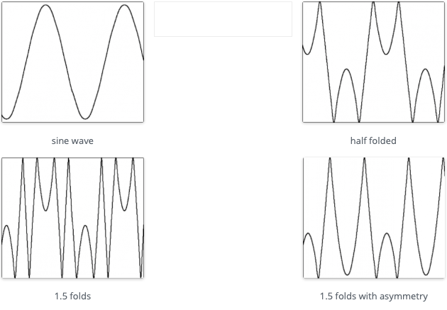
Wavefolding is a process which was originally used in the Buchla 259 complex waveform generator, a module from the Buchla 200 electronic music box and later in Serge synthesizers. It is a waveshaping function which “folds” back any input signal which exceeds a threshold. Usually there are positive and negative thresholds, so that both sides of the signal are folded. It is easiest to show this graphically.

You can see how the sine wave is reversed on the top and bottom of the waveform and that this fold is reversed again in the 1.5x example when reaching the opposite threshold. The asymmetrical example is synthesized by adding a negative constant to the signal so that the negative threshold is reached before the positive one.

Wavefolding adds many new harmonics to any oscillator. This was a powerful technique on analog synthesizers as rich sounds could be created with just a handful of opamps and diodes.

Implementation

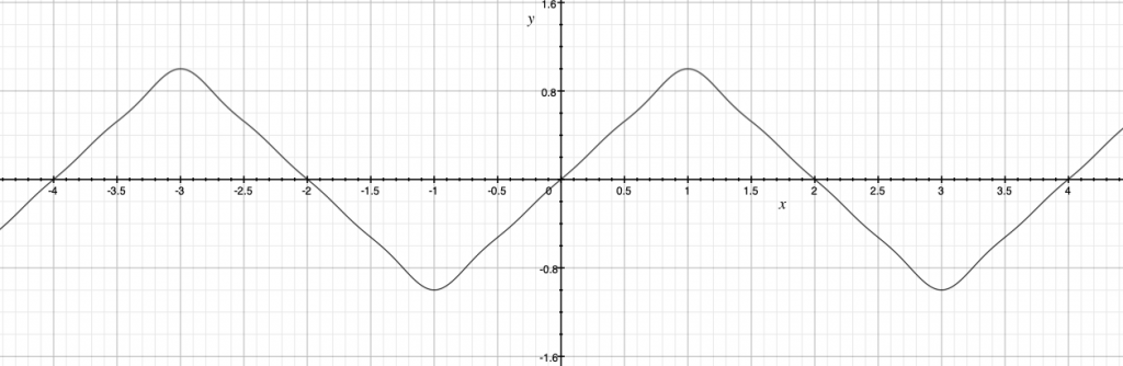
Wavefolding can be implemented by using a transfer function which reverses the signal at the positive and negative limits (-1 and 1), and again at -3, 3, -5, 5 and so on. The slope of this function should always be 1 or -1 (reversal). It is essentially a triangle wave. Here is a triangle wave approximated with it’s first 4 harmonics.

The incoming signal provides an index into the x axis, and the y axis is the output of the wavefolder. This can be implemented with a single cycle wavetable and a wrap function, or we can compute this directly from the modified triangle equation, sending the signal into x. As the signal is amplified beyond a gain of 1.0, wavefolding will start.

y_(x) = cos(.5\pi x) - \frac{1}{9} cos(1.5\pi x) + \frac{1}{25} cos(2.5\pi x) - \frac{1}{49} cos(3.5\pi x)

Here is some example C code which uses the direct synthesis method.

WaveFolder(float *input, float *output, long samples, float gain, float offset) 
{
  int sample;
  float pi = 3.141592653589793;

  // iterate through the samples in the block
  for(sample = 0; sample<samples; sample++) 
  {
    // scale the input signal by gain and add offset
    ingain = (gain * *(input+sample)) + offset;

     *(output+sample) = cos(0.5 * pi * ingain)
        - 1.0/9.0 * cos(1.5 * pi * ingain)
        + 1.0/25.0 * cos(2.5 * pi * ingain)
        - 1.0/49.0 * cos(3.5 * pi * ingain);
  }
}

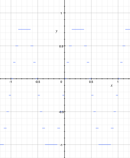
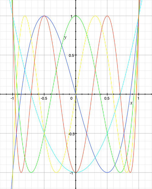
The chebyshev polynomials are often used in synthesis to create harmonics from sinusoidal components. Five of the polynomials (degree 2 to 6) are plotted below:

degree 2 (light blue): y = 2x^2 - 1
degree3 (blue): y = 4x^3 - 3x
degree 4 (green): y = 8x^4 - 8x^2 + 1
degree 5 (yellow): y = 16x^5 - 20x^3 + 5x
degree 6 (red): y = 32x^6 - 48x^4 + 18x^2 - 1

These transfer functions are used for input signals within the range of -1 to 1, as the output of these functions rapidly increase beyond that. The gain on the input signal should be limited to 1.0. Because of the curved reversals in the chebyshev polynomials, they can be used as smooth wavefolders. As the input signal increases, the output quickly goes to the maximum value and wraps back. This smoothed wavefolding creates higher harmonics based on the original harmonics.

Furthermore, the chebyshev polynomials have an interesting effect on sine waves. When the sine wave is at a low level, the degree 3 polynomial will reproduce the sine wave, as the sine wave increases in volume, the 3rd harmonic will appear, and at full volume, the fundamental will disappear.

degree	harmonic transformation
2	0 – 2
3	1 – 3
4	0 – 2 – 4
5	1 – 3 – 5
6	0 – 2 – 4 – 6

One should note that if these are applied to harmonically rich waveforms or samples, every harmonic in the source signal will be multiplied. In this context, these waveshapers will create harmonic distortion and sound much like a distorted amplifier. Also, the even polynomials contain a DC component (harmonic 0). For practical use it may be necessary to remove the DC offset with a high pass filter.

When working with sine waves, the chebyshev waveshapers can be very effectively used for direct harmonic synthesis. They can also be used to replace the sine wave oscillators in additive synthesis or frequency modulation to extend those synthesis techniques.

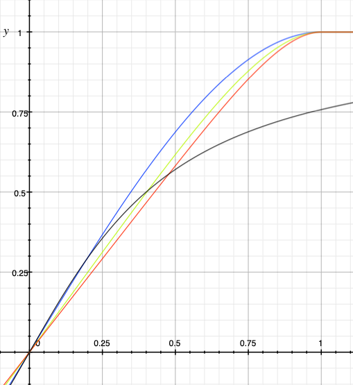
In our section on amplitude, saturation using a cubic polynomial was shown. Alternatively polynomials of larger degree than 3 can be used. Consider the following:

y = -0.25x^5 + 1.25x

y = -0.16666x^7 + 1.16666x

The advantage of these higher degree functions is that the signal remains undistorted at larger amplitudes, and also that the gain (the slope of the saturation function) is closer to one. The disadvantage is that distortion appears more quickly when the signal reaches the saturation point.

From the plot above, the atan saturation is shown to be less linear at lower signal values. On the other hand, it goes much more slowly into saturation. For this reason, many find it to sound “warmer” than the polynomial functions.

These saturation functions are more generally known as transfer functions, or and in synthesis they are known as waveshapers. Waveshapers can be used to distort a waveform in musical ways. For instance, brass synthesis often uses a saturation waveshaper, as it makes the tone brighter when it gets louder.

Any arbitrary shape can be used in a waveshaping transfer function, and certain early digital synthesizers (Buchla 400, Buchla Touché) did just this. Discontinuous functions have been used to emulate certain fuzz pedals, or to create decimation effects (aka bitcrushing). In the next few sections we will look at a few of the types of waveshaping.

An ADSR (attack, decay, sustain, release) envelope is used to shape a note. Typically it is used to control the gain of the note, but can also be used to control amount of brightness, bass, distortion, tremolo, vibrato, or anything else that varies over the course of a note.

There are shorter and longer variations of an ADSR. The AR envelope is often used for percussive sounds. The ASR envelope is used when there is no transient at the start of a note. The DADSR envelope has a delay stage at the beginning, and is used for parameters that don’t begin immediately at the start of a note (vibrato typically begins a little after the start of the note). There can be envelopes with more stages, and many hardware synths have envelopes of 8 or more stages.

Implementation

To implement an ADSR envelope, one has to keep track it’s state. Then the envelope can do the appropriate thing for the state.

• Attack: during this state the envelope level will rise from 0.0 to 1.0 over the attack time. The envelope enters this state when the note starts. When the level reaches 1.0, the state will switch to decay.
• Decay: during this state the envelope level will drop from 1.0 to the sustain level over the decay time. When the envelope reaches the sustain level, the state will switch to sustain.
• Sustain: during this state the envelope level will be the sustain level. The envelope will stay in this state until the note ends (the key is lifted).
• Release: during this state the envelope level will drop from it’s current level to 0.0 over the release time. The envelope enters this state when the note stops (this can be during the attack, decay or sustain state).
• Off: This state is entered from the release state when the envelope level reaches 0.0. During this state, the envelope level stays at 0.0.

The code for an envelope which responds to MIDI velocity (1 to 127, note on, 0 is note off) could look like this. Notice what conditions cause the envelope to change from one state to another. Also notice that release can be entered from any state. This code should be improved in order to avoid divide by zero errors.

enum envState {
    kAttack,
    kDecay,
    kSustain,
    kRelease,
    kOff
};

long state = kOff;
float increment;
float envelopeLevel;
float samplerate = 44100;


float ADSR(float MIDIvelocity, float attacktime, float decaytime, float sustainlevel, float releasetime)
{
    switch(state)
    {
    case kOff:
        envelopeLevel = 0.0;
        if(MIDIvelocity > 0)
        {
            increment = (1.0 - envelopeLevel)/(attacktime * samplerate);
            state = kAttack;
        }
        break;
    case kAttack:
        if(envelopeLevel >= 1.0)
        {
            increment = (sustainLevel - envelopeLevel)/(decaytime * samplerate);
            state = kDecay;
        }
        break;
    case kDecay:
        if(envelopeLevel <= sustainlevel)
        {
            increment = 0.0;
            state = kSustain;
        }
    case kRelease:
        if(envelopeLevel <= 0.0)
        {
            envelopeLevel = 0.0;
            state = kOff;
        }
    }
    envelopeLevel = envelopeLevel + increment;
    if(MIDIvelocity = 0 && (state != kOff || state != kRelease)
    {
        increment = envelopeLevel/(releasetime * samplerate);
        state = kRelease;
    }
    // use MIDI velocity to change volume of envelope
    return(envelopeLevel * MIDIvelocity/127.0);  
}