Monthly Archives: November 2019

Two Operator Frequency Modulation

Frequency Modulation is a synthesis technique that all should be familiar with. FM synthesis was invented by John Chowning in 1968, and subsequently the most commercially popular digital synthesis method. It involves at least 2 operators (sine oscillator with amplifier), in which one is the modulator and the other is the carrier (the operator being modulated, as well as the one that is heard).

The theory of FM synthesis can be found in Chowning’s article “The Synthesis of Complex Audio Spectra by Means of Frequency Modulation”. Breifly, frequency modulation acts somewhat like amplitude modulation in that upper and lower sidebands are created around the carrier frequency. These sidebands are separated from the frequency of the carrier by the frequency of the modulator, so that they appear at f_{car} + f_{mod} and f_{car} - f_{mod}. What separates FM from AM is that additional sidebands appear at multiples of the modulator frequency, and increased depth of modulation increases the strength of higher sidebands. Also when f_{car} - n*f_{mod} drops below 0Hz, it reflects around 0Hz with a phase inversion. As with AM, a simple harmonic relation between the carrier and modulator will create a more consonant sound Finally, multiple carriers and modulators can be used to specify a spectrum in more detail, and modulation feedback can be used to create noise and chaotic oscillation..

simple two operator frequency modulation

Implementation

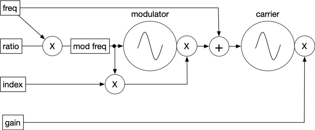
One of the attractive aspects of two operator FM synthesis is that this very straightforward and seemingly simple structure can intuitively create many timbres. The index parameter acts very much like a brightness control, a ratio of 1 will synthesize all harmonics, a ratio of 2 will create odd harmonics, and higher ratios further separate the overtones. The only limit to index and ratio is the Nyquist frequency.

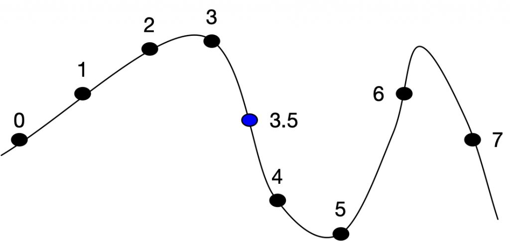
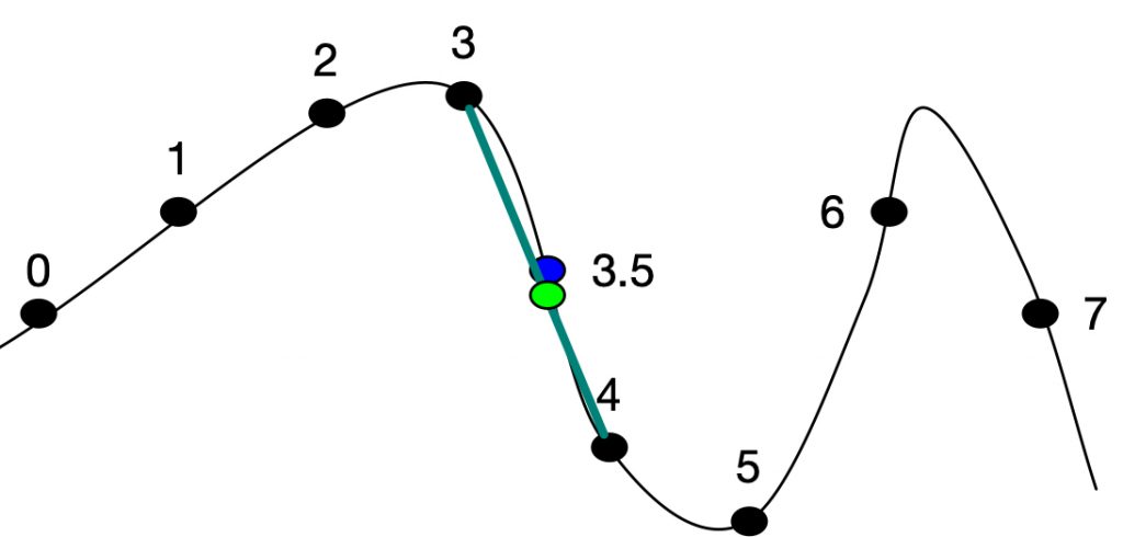
In C, two table lookup oscillators are used. In practice, interpolation would be used in these oscillators to reduce quantization noise.

// the samplerate in Hz
float sampleRate = 44100;
// initial phase
float phaseCar = 0.0;
float phaseMod = 0.0;
long tableSize = 8192;
long tableMask = 8191;
float sineTab[8192];

void InitTables(void)
{
  // create sineTab from sin()
  for(i = 0; i < tableSize; i++)
  {
    sineTab[i] = sin((6.283185307179586 * i)/tableSize);
   }
}


void TwoOpFM(float *input, float *output, float frequency, float ratio, float index, float gain, long samples)
{
    long sample;
    float phaseIncCar, phaseIncMod;
    float carrier, modulator;
    // calculate for each sample in a block
    for(sample = 0; sample < samples; sample++)
    {
      // get the phase increment for this sample
      // frequency of modulator is frequency of carrier * ratio
      phaseIncMod = (frequency * ratio)/sampleRate;
        
      // calculate the waveforms
      modulator = sineTab[(long)(phaseMod * tableSize)];
      phaseIncCar = (frequency + (modulator * frequency * ratio * index))/sampleRate;
      carrier = sineTab[(long)(phaseCar * tableSize)];        
      *(output+sample) = carrier * gain; 

        // increment the phases
        phaseMod = phaseMod + phaseModInc;
        phaseCar = phaseCar + phaseIncCar;
       if(phaseMod >= 1.0)
            phaseMod = phaseMod - 1.0;
       // phaseCar can get large fast and can go negative
       // must be kept between 0 and 1
        while(phaseCar >= 1.0)
            phaseCar = phaseCar - 1.0;
        while(phaseCar < 0.0)
            phaseCar = phaseCar + 1.0;
  }
}
2 op FM with random index and ratio

Multiple Carriers, Feedback FM and further

One could easily add more to this simple network. One of the common additions is that of a second carrier with it’s own index of modulation. This can be used to simulate formants, or increase upper harmonics without increasing middle harmonics.

Feedback is often used in small amounts to create a bit of noise for the attack of the note. This can be done by adding a modulation path from the carrier to the modulator. There will be an additional sample delay in this feedback, but this technique can create a wide variety of noise depending on the index and frequency.

Finally, there are many, many papers on synthesis with FM, as well as commercial instruments that have some very expressive FM patches. It is well worth it to study these patches and techniques.

Single Sideband AM

Single sideband amplitude modulation shifts the frequency either upward or downward, but not both directions (as in AM). This technique is based on the trigonometric identity we used earlier. Shifting a cosine up simply takes half of a complex multiplication.

cos(\alpha+\beta)=cos(\alpha)cos(\beta)−sin(\alpha)sin(\beta)

Alpha and beta represent the frequencies of the signal sources. Each of these frequencies requires a cosine and sine oscillator pair. By subtracting the sin() product from the cos() product, a frequency shifted (alpha+beta) oscillator is synthesized. If the products are summed, a downward (alpha-beta) oscillator is synthesized. As cosine and sine are separated by 90 degrees, it is simple enough to create a cosine/sine pair from a sinusoidal oscillator – simply add 90 degrees to the phase of the oscillator to create the second of the pair.

However, single sideband AM is more often used to frequency shift sampled signals. To do this, it is useful to consider the sample as a sum of multiple sinusoidal oscillators. To perform SSB AM, the original sample as well as a 90 degree phase shifted sample is needed. Phase shifting all of the sinusoidal components of a sample 90 degrees can be done with a type of allpass filter called a Hilbert transformer. If well designed, a Hilbert transformer will shift most frequencies 90 degrees, and will maintain this phase shift until close to 0Hz and the Nyquist frequency. Many implementations have two outputs which are 90 degrees apart, but not in phase with the original sample.

Frequency shifting with a hilbert transformer.

Calculating coefficients for a Hilbert transformer is beyond the scope of this class, but one could read articles by Scott Wardle or Dan Harris, Edgar Berdahl and Jonathan Abel for more information in this area.

Implementation

There are several open source Hilbert transformers in popular audio software. One is in Miller Puckette’s Pure Data, and is implemented as 2 pairs of biquad filters (a biquad filter was used in the earlier second order allpass filter example). It is based on a 4X synthesizer patch by Emmanuel Favreau. The other is in the Csound source code, designed by Sean Costello and based on data from Bernie Hutchins.

The difference equations for the Favreau Hilbert transformer are:

\scriptsize x1[n]=x3[n]=in\\x2[n]=y1[n]=0.94657x1[n]-1.94632x1[n-1]+x1[n-2]+1.94632y1[n-1]-0.94657y1[n-2]\\ outsin = y2[n] = 0.06338x2[n]-0.83774x2[n-1]+x2[n-2]+0.83774y2[n-1]-0.06338y2[n-2]\\x4[n]=y3[n]=-0.260502x3[n]+0.02569x3[n-1]+x3[n-2]-0.02569y3[n-1]+0.260502y3[n-2]\\ outcos = y4[n] = 0.870686x4[n]-1.8685x4[n-1]+x4[n-2]+01.8685y4[n-1]-0.870686y4[n-2]

Notice that this specifies two pairs of allpass filters in which each pair is in series. The C code follows directly from these equations.

// the samplerate in Hz
float sampleRate = 44100;
// initial phase
float phase = 0.0;
long tableSize = 8192;
long tableMask = 8191;
float sineTab[8192];
float x1[3], x2[3], x3[3], x4[3];
float y1[3], y2[3], y3[3], y4[3];

void InitTables(void)
{
  // create sineTab from sin()
  for(i = 0; i < tableSize; i++)
  {
    sineTab[i] = sin((6.283185307179586 * i)/tableSize);
   }
}


// 4 biquad filters
void Hilbert(float input, float *sinout, float *cosout)
{
  x1[0] = x3[0] = input;
  x2[0] = y1[0] = 0.94657*x1[0] − 1.94632*x1[1] + x1[2]
    + 1.94632*y1[1] − 0.94657*y1[2];
  y1[2] = y1[1];
  y1[1] = y1[0];
  x1[2] = x1[1];
  x1[1] = x1[0];
  *sinout = y2[0] = 0.06338*x2[0] − 0.83774x2[1] + x2[2] 
    + 0.83774*y2[1] − 0.06338*y2[2];
  y2[2] = y2[1];
  y2[1] = y2[0];
  x2[2] = x2[1];
  x2[1] = x2[0];

  x4[0] = y3[0] = -0.260502*x3[0] + 0.02569*x3[1] + x3[2] 
    - 0.02569*y3[1] + 0.260502*y3[2];
  y3[2] = y3[1];
  y3[1] = y3[0];
  x3[2] = x3[1];
  x3[1] = x3[0];
  *cosout = y4[0] = 0.870686*x4[0] − 1.8685*x4[1] + x4[2] 
    + 1.8685*y4[1] − 0.870686y4[2];
  y4[2] = y4[1];
  y4[1] = y4[0];
  x4[2] = x4[1];
  x4[1] = x4[0];
}
void FreqShift(float *input, float *output, float frequency, float ratio, float ringGain, float sineGain, float squareGain, long samples)
{
    long sample;
    float phaseInc;
    float sinOsc, cosOsc, sinSamp, cosSamp;
    // calculate for each sample in a block
    for(sample = 0; sample < samples; sample++)
    {
        // get the phase increment for this sample
        phaseInc = frequency/sampleRate;

        // calculate the waveforms
        sinOsc = sineTab[(long)(phase * tableSize)];
        cosOsc = sineTab[((long)(phase+0.25 * tableSize))%tableMask];
        Hilbert(*output+sample, &sinSamp, &cosSamp);

        *(output+sample) = sinSamp * sinOsc - cosSamp * cosOsc; 

        // increment the phases
        phase = phase + phaseInc;
        if(phase >= 1.0)
            phase = phase - 1.0;
  }
}
“Walk This Way” break shifted from 1000Hz up to 200Hz down

Amplitude Modulation

Introduction

Amplitude Modulation (aka ring modulation) is one of the simplest synthesis techniques to implement, but one of the lesser used techniques. AM uses the multiplication of two signals to create new harmonics. The product will contain the sum and difference of all of the harmonics in the original waveforms. This comes from the combinations of the phase change in the original waveforms. If you take the difference of two trigonometric angle sum and difference identities you can see how the new frequencies are derived from the multiplied sines.

cos(\alpha - \beta) = cos(\alpha)cos(\beta) + sin(\alpha)sin(\beta) \\ cos(\alpha + \beta) = cos(\alpha)cos(\beta) - sin(\alpha)sin(\beta) \\ cos(\alpha - \beta) - cos(\alpha + \beta) = 2*sin(\alpha)sin(\beta) \\ sin(\alpha)sin(\beta) = \frac{1}{2}*(cos(\alpha - \beta) - cos(\alpha + \beta))

As the frequencies are being shifted with sum and difference, these new harmonics can easily lose any harmonic relation they had in the original signals. For example, if a waveform with related harmonics of 100Hz, 200Hz and 500Hz is modulated by a 96Hz sine, the new harmonics will be at 4Hz, 104Hz, 196Hz, 296Hz, 404Hz and 596Hz. There are no simple harmonic relations in the new tone.

96Hz sine * 100,200&500Hz sine
“Walk This Way” break * sine sweep from 1k to 0Hz

Amplitude Modulation Techniques

AM can be configured in several ways to get more consonant results. The C code below will show how to achieve the following three methods.

  • By restricting the frequencies used in AM, a more useful result is obtained. If simple harmonic relations are maintained between the two source waveforms, harmonic relations will be maintained in the product.
  • The original waveforms can be reintroduced into the output by adding two parameters. This can be very useful if one of the sources isn’t sinusoidal. y(t) = \alpha*(sin(\omega_1 t)*sin(\omega_2 t) + \beta*sin(\omega_1 t) + \gamma*sin(\omega_2 t))
  • A simple harmonic tone generator can be created using feedback and self modulation.

Implementation

AM is usually implemented with a simple multiply and two source signals. Our first C example will create an AM oscillator with internal sqaure and sine wave oscillators. It will also implement gain parameters for the original waveforms.

// the samplerate in Hz
float sampleRate = 44100;
// initial phase
float phaseSin, phaseSqu = 0.0;
long tableSize = 8192;
long tableMask = 8191;
float squareTab[8192];
float sineTab[8192];

void InitTables(void)
{
  // create sineTab from sin() and squareTab from 11 first harmonics of square wave
  for(i = 0; i < tableSize; i++)
  {
    sineTab[i] = sin((6.283185307179586 * i)/tableSize);
    squareTab[i] = sin((6.283185307179586 * i)/tableSize);
    squareTab[i] += sin((6.283185307179586 * i * 3.0)/tableSize)/3.0;
    squareTab[i] += sin((6.283185307179586 * i * 5.0)/tableSize)/5.0;
    squareTab[i] += sin((6.283185307179586 * i * 7.0)/tableSize)/7.0;
    squareTab[i] += sin((6.283185307179586 * i * 9.0)/tableSize)/9.0;
    squareTab[i] += sin((6.283185307179586 * i * 11.0)/tableSize)/11.0;
    squareTab[i] += sin((6.283185307179586 * i * 13.0)/tableSize)/13.0;
    squareTab[i] += sin((6.283185307179586 * i * 15.0)/tableSize)/15.0;
    squareTab[i] += sin((6.283185307179586 * i * 17.0)/tableSize)/17.0;
    squareTab[i] += sin((6.283185307179586 * i * 19.0)/tableSize)/19.0;
    squareTab[i] += sin((6.283185307179586 * i * 21.0)/tableSize)/21.0;
  }
}

void RingOsc(float *input, float *output, float frequency, float ratio, float ringGain, float sineGain, float squareGain, long samples)
{
    long sample;
    float phaseIncSin, phaseIncSqu;
    float sinSamp, squSamp;
    // calculate for each sample in a block
    for(sample = 0; sample < samples; sample++)
    {
        // get the phase increment for this sample
        phaseIncSqu = frequency/sampleRate;
        phaseIncSin = phaseIncSqu * ratio;
        // calculate the waveforms
        sinSamp = sineTab[(long)(phaseSin * tableSize)];
        squSamp = squareTab[(long)(phaseSqu * tableSize)];

        // mix the output from ring, sine and square
        *(output+sample) = sinSamp * squSamp * ringGain + squSamp * squareGain
          + sinSamp * sineGain; 

        // increment the phases
        phaseSin = phaseSin + phaseIncSin;
        if(phaseSin >= 1.0)
            phaseSin = phaseSin - 1.0;
        phaseSqu = phaseSqu + phaseIncSqu;
        if(phaseSqu >= 1.0)
            phaseSqu = phaseSqu - 1.0;
    }
}
square * sine ring oscillator with ratio of 3 and modulation of square and sine gain

As stated earlier, a simple harmonic oscillator can be made by using a single sinewave oscillator, AM and feedback. Feedback needs to be kept under 1.0 or the algorithm will become unstable. As the feedback gain increases, more and more harmonics will be added. A small offset needs to be added to the feedback to give the sound an initial gain. Not a very rich technique, but worth knowing….

// the samplerate in Hz
float sampleRate = 44100;
// initial phase
float phase = 0.0;
float fbSamp;
long tableSize = 8192;
long tableMask = 8191;
float sineTab[8192];

void InitTables(void)
{
  // create sineTab from sin()
  for(i = 0; i < tableSize; i++)
  {
    sineTab[i] = sin((6.283185307179586 * i)/tableSize);
  }
}

void RingFBOsc(float *input, float *output, float frequency, float feedback, long samples)
{
    long sample;
    float phaseInc;
    float sinSamp, squSamp;

    if(feedback > .95) feedback = .95;
    // calculate for each sample in a block
    for(sample = 0; sample < samples; sample++)
    {
        // get the phase increment for this sample
        phaseInc = frequency/sampleRate;
        // calculate the waveforms
        sinSamp = sineTab[(long)(phase * tableSize)];

        // ring modulate with last output * feedback
        fbSamp = sinSamp * ((fbSamp * feedback) + 0.1)
        *(output+sample) = fbSamp; 

        // increment the phase
        phase = phase + phaseInc;
        if(phase >= 1.0)
            phase = phase - 1.0;
    }
}
random bass line with single oscillator feedback AM modulation

Delay Applications

Many characteristic effects can be created by configuring the delay in the right way. I will describe how to get some of these effects.

Comb Filtering

For comb filtering, the time needs to be very short, from about 40ms to .1ms. An exponential time control will help in tuning specific pitches. To get the filter to ring, the feedback should be very high, about 90% and above (even above 100%). There should be less compression (or no compression) in the feedback loop. Saturation in the feedback loop can make this effect really stand out.

Flanging

Flanging can be achieved by starting with the comb filter settings above. Modulate the time slowly (1/10th to 2Hz) with a triangle wave from the delay’s minimum time to 10 – 40ms. A low pass filter in the feedback loop can change the timbre of the flange effect.

Multitap Echo

A “tap” is a secondary output of the same delay with a different time. Implementation is fairly simple – add multiple reads of the delay buffer, each with a different delay time. These multiple outputs can create a rhythmic pattern, and each delay output could have a separate gain control. Mix all of the outputs, and be careful not to distort as the taps are summed.

Chorusing

This can be done with one or many taps. The delay times are modulated without much depth around 30ms (so from 29 to 31ms is typical). Modulation is typically done with a sine wave at a low frequency (like the flanger). If multiple taps are used, each one should be modulated by a different phase sine wave, and if possible, output to different spatial locations. Feedback is typically low when chorusing, unless a “seasick” pitch warble is desired.

Loop/Freeze

Delay looping is not the same as a full feature looper, but can be used for some loop applications. Simply set the feedback to 100% (1.0) and the input gain to 0.0, and the sound will be held and repeated.

Delay With Feedback

Adding feedback to a delay is fairly straightforward: output = input + delayouput * feedback , where feedback ranges from 0.0 to 1.0 (and often over 1.0). Adding a feedback path is what creates multiple echoes, with a naturally exponential decay. A typical implementation is to send the delay output to an input/output mix, and apply feedback gain before the delay output is mixed with the input. In this configuration, mix determines the balance of the delay and the input, and feedback controls the decay of each echo.

typical delay configuration with feedback and wet./dry mix.

Note that delay output * feedback + input, has a gain of 1.0 + feedback. This will drive the delay into clipping when there are input signals over 0.5. There are a number of options to control the gain (keep it at 1.0): gain reduction based on feedback, compression, saturation, or a combination of the these. Simple gain reduction would place a gain element before the delay input so that the overall gain is reduced as the feedback increases.

delayinput = (input + delayoutput * feedback) * (1.0/(1.0 + feedback))

This is the cleanest sounding approach, but is sometimes felt to be too “clinical”. A combination of compressor and saturator is more typically used.

compression after feedback/input mix to keep signal under 1.0

This compressor will measure the level before the delay input and apply a gain lower than 1.0 to control the signal. This gain can be applied before the delay input or to the feedback signal.

Finally, when implementing any feedback network, there is a danger of DC offset building up. If using feedback higher than 1.0 this is especially likely. A DC blocking filter (a high pass at a subsonic frequency) in the feedback path should be tuned to remove any DC offset without negatively affecting low frequencies.

Implementation

The addition of feedback and wet/dry mix to a delay is fairly simple. Saturation can be added before the delay input. A compressor can be implemented as it was in the earlier section, but in the case where the threshold is fixed and the amount of gain reduction needed is known, a gain table can be kept in memory, or a polynomial can be used to calculate gain. This polynomial can be created by curve fitting through the known gain reduction points (polyfit in MatLab can do this, as can several online solvers).

y=1.60154 – 1.60573x + 0.88839x^2 – 0.18048x^3 (gain of 1 at .5, gain of .5 at 2)
// this code uses the earlier linear interpolation method
long writePointer, delayMask;
float *delayBuffer;
float delayTime;
float sampleRate = 48000.0f;
float peak;

void DelayInit(long delaySize)
{
  delayBuffer = new float[delaySize];
  delayMask = delaySize - 1;
  writePointer = 0;
  delayTime = 0.0f;
  peak = 0.0f;
}

void DelayTerm(void)
{
  delete[] delayBuffer;
}

void Delay(float *input, float *output, long samples, float time, float feedback, float mix)
{
  float readPointer; 
  long readPointerLong, i; 
  float fraction; 
  float x0, x1, out, in, rect;
  delayTimeInc;

  // find increment to smooth out delayTime
  delayTimeInc = (time - delayTime)/samples;
  for(i = 0; i < samples; i++)
  {
    in = *(input+i);
    // linear interpolated read
    readPointer = writePointer + (delayTime*sampleRate); 
    readPointerLong = (long)readPointer; 
    fraction = readPointer - readPointerLong; 
    // both points need to be masked to keep them within the delay buffer 
    x0 = *(delayBuffer + (readPointerLong & bufferMask)); 
    x1 = *(delayBuffer + ((readPointerLong + 1) & bufferMask)); 
    out = x1 + (x2 - x1) * fraction;
    // wet/dry mix
    *(output+i) = out * mix + in * (1.0 - mix);
    
    // add feedback output to input
    rect = in = in + feedback * out;

    // rectify input for simple peak detection
    if(rect < 0.0) rect = rect * -1.0;
    // if the signal is over the peak, use one pole filter for quick fade of peak to signal
    if(peak < rect)
      peak = peak + (rect - peak) * 0.9f;
    // otherwise fade peak down slowly
    else
      peak *= 0.9999f;
    // polynomial compression
    // if feedback goes up to 1.0, a maximum peak of 2.0 is possible
    if(peak > 2.0)
      peak = 2.0;
    else if(peak < 0.5f) 
      peak = 0.5f;
    in = in * (1.601539 - (1.605725 * peak) 
               + (0.8883899 * peak * peak)
               - (0.180484 * peak * peak * peak));
    // now it can go in the delay
    *(delaybuffer + writePointer) = in; 
    // move the write pointer and wrap it by masking
    writePointer--; 
    writePointer &= delayMask;
    // smooth the delayTime with the increment
    delayTime = delayTime + delayTimeInc;
  }
  delayTime = time;
}


Fractional Delay And Smoothed Time Control

Introduction

The delay code in the previous posting quantizes the delay value to the sample. This can cause problems when modulating the delay time, as many modulated delay effects (doppler shift, comb filtering, chorusing, flanging) depend on sub-sample time accuracy. It is also necessary to smooth the time control to decrease parameter change noise (aka “zipper noise”). When adjusting the delay time with a mouse (in a plugin or app), the time parameter will only be updated once per sample block. This sporadic parameter change needs to be smoothed through interpolation or other filtering techniques. Finally, if your delay time is being controlled by an analog control, there is often noise or jitter in this control. This also needs to be smoothed. In this section a few of these techniques will be presented.

Fractional Delay

A fractional delay estimates possible values between actual samples, by using a interpolation or curve fitting technique.

possible curve for 7 samples

If the sample rate is 48k, and a delayed sample at time .0729ms is needed, the sample at location 48 * 0.0729 = 3.5 is needed. Of course, there is no sample 3.5, but an estimate can be made. There are several common techniques to finding this value (these are the same techniques used in a table lookup oscillator):

  • truncation
  • rounding
  • linear interpolation
  • hermite interpolation
  • other interpolation functions

Truncation is the simplest of these techniques. Simply truncate any number right of the decimal point and 3.5 becomes 3. This is the fastest, and worst sounding method. Rounding involves finding the closest integer. It is the same as adding 0.5 to the floating point sample number and then truncating – 3.5 becomes 4. It sounds as bad as truncation but involves more computation. Linear interpolation is a much better estimate. This involves calculating the value between 3 and 4 by a simple crossfade.

The value given by linear interpolation will have error, but is much better than the value given by truncation.

Even more accurate are curve fitting functions like the 4 point hermite cubic interpolator which is discussed in great detail in the oscillator section of this website. It uses the 4 points around 3.5 (2, 3, 4, 5) to estimate the value at 3.5 giving more weight to points 3 and 4. There are many interpolators, using more or less points, and with varying accuracy and CPU performance. A good discussion of these is in this paper by Olli Neimitalo.

Implementation

To implement linear interpolation, the sample points around the fractional point are needed. The the first sample number (3 in the example) is subtracted from the desired sample number (3.5) to get the fraction (0.5). We can use this fraction to estimate the value at 3.5: y = x_{3} * (1 - frac) + x_{4} * frac or y = x_{3} + (x_{4} - x_{3}) * frac .

// The sample reading code is modified for linear interpolation

float readPointer;
long readPointerLong;
float fraction;
float x0, x1;

readPointer = writePointer + (delayTime*sampleRate);
readPointerLong = (long)readPointer;
fraction = readPointer - readPointerLong;
// both points need to be masked to keep them within the delay buffer
x0 = *(delayBuffer + (readPointerLong & bufferMask));
x1 = *(delayBuffer + ((readPointerLong + 1) & bufferMask));
outputSample = x1 + (x2 - x1) * fraction;

Using the hermite polynomial is a little more involved, temporary variables c0 – c4 are used to make the code easier to read. This is using James McCartney’s code from musicdsp.org:

// The sample reading code is modified for cubic interpolation

float readPointer;
long readPointerLong;
float fraction;
float xm1, x0, x1, x2;
float c0, c1, c2, c3;

readPointer = writePointer + (delayTime*sampleRate);
readPointerLong = (long)readPointer;
fraction = readPointer - readPointerLong;
// all points need to be masked to keep them within the delay buffer
xm1 = *(delayBuffer + ((readPointerLong - 1) & bufferMask))
x0 = *(delayBuffer + (readPointerLong & bufferMask));
x1 = *(delayBuffer + ((readPointerLong + 1) & bufferMask));
x2 = *(delayBuffer + ((readPointerLong + 2) & bufferMask));

c0 = x0;     
c1 = 0.5 * (x1 - xm1);     
c3 = 1.5 * (x0 - x1) + 0.5f * (x2 - xm1);     
c2 = xm1 - x0 + c1 - c3;     

outputSample = ((c3 * fraction + c2) * fraction + c1) * fraction + c0;

Smoothed Time Control

When processing samples in blocks, it is necessary to provide an interpolated delay time parameter for every sample. We can do this by simply calculating the change in parameter value for each sample as follows.

float currentDelayTime;

void Delay(float *input, float *output, float delayTime, long samples)
{
  float delayTimeIncrement;
  long i;

  delayTimeIncrement = (delayTime - currentDelayTime)/samples;
  
  for(i = 0; i < samples; i++)
  {
    // DELAY CODE GOES HERE USING currentDelayTime
    currentDelayTime = currentDelayTime + delayTimeIncrement;
  }
  currentDelayTime = delayTime;
}

This takes care of smoothing out parameter change between blocks, however, additional smoothing could be needed for external controllers. A mouse position can be updated as slowly as 60 times a second. Other external sources (knobs, MIDI, network) can also have noise or jitter. Generally it is necessary to design a smoothing filter that works for each source, smoothing the jitter, but quick enough to feel responsive. A simple low pass filter is one common approach.

currentTimeControl  = 0.99 * (currentTimeControl - timeControl) + timeControl;
delayTime = currentTimeControl;

The coefficient (0.99) can be varied for responsiveness. At 48k, this comes within 1% of the new control position in just under 10ms.

Dopper Shift Limiting

The other factor one might consider, especially when there is a large range for the delay time, is to limit the change of delay time per sample. If the delay time moves quickly across a large time span (i.e. from 10ms to 5s), it can create high frequency doppler shift. In this case, it is helpful to limit the change by sending it through a saturation function (a sigmoid, s shaped, function). In the following code this is done with atan().

float delayTimeChange = delayTime - delayTimeLimited; 
delayTimeChange = 4.0 * atan(delayTimeChange * 0.25);
delayTimeLimited += delTimeChange;

The factors 0.25 and 4.0 are chosen here to allow the delay time change to be fairly linear under 1.0 (1 sample of delay time change per 1 sample played), but increasingly limited as so that the delay time never changes more than 2π per sample. This factor is a doppler shift of about 2.5 octaves. Changing the factors around atan() will change this doppler shift limit.

Introduction: Single Echo Delay

Introduction

Delay effect design draws on a number of previously explored techniques. Wavetable interpolation will be used to read samples from the delay. Compression and saturation will be used to maintain the gain within the feedback loop. Filtering will be used to remove high or low frequencies from the echoes. A delay starts with a fairly straightforward design, but becomes complex with the integration of these techniques, and gathers its individual character as design decisions are made.

Design

To create a delay, we need a sample buffer to hold audio until the delayed signal is played. Input samples will continually be written to this buffer, and output samples will continually be read from this buffer. To do this, point the input sample to a starting location, write the sample, and move the input pointer one sample over. The output pointer is positioned relative to the input pointer, with the delay time in samples separating them. If the delay time is 1.4 seconds, and the sample rate is 48k, the separation between input and output pointer is 1.4 x 48000 or 67200 samples.

If unlimited storage is available, the input pointer and output pointer could move indefinitely. A large storage space could be used: a 1TB flash drive could run a delay at 48k/32 bit for 30 days before running out of memory. However, much smaller and faster memory is more typically used for the sample buffer. Because of this, it is typical to reuse the memory – after the input pointer reaches the last sample, it resets to the first sample. This is called a circular buffer. A large enough buffer is needed for the longest delay time desired. For a 42 second delay, with a sample rate of 48k, enough memory to hold 42 * 48,000  or 2,016,000 samples is needed. For sample addressing convenience (discussed later), we will use the nearest power of 2. In this case it is 2^21 or 2,097,152 samples.

Implementation

On embedded processors, it is typical to use physical memory for the circular buffer. In that case we could just use an array declaration. For a plugin or app, memory allocation is necessary. The functions malloc (C) or new (C++) would be used to create the sample buffer.

// C example of delay memory allocation
float *delayBuffer;
long delaySize, delayMask;
delaySize = 2097152;
delayMask = delaySize - 1;
delayBuffer = (float *)malloc(delaySize * sizeof(float));

Pointer arithmetic is used to determine the memory location to write the input sample. After the sample is written, writePointer is moved one sample. In the diagrams above writePointer is incremented. However, it makes our program simpler if writePointer is decremented. This is because readPointer is calculated by adding the delay in samples to writePointer. After decrementing, a bitwise AND is used to maintain the circular buffer (to make sure writePointer is between 0 and delaySize).

// C example of putting sample in delayBuffer, 
// decrementing and wrapping writePointer
*(delayBuffer + writePointer) = inputSample;
writePointer--;
writePointer &= delayMask;

To complete our echo, the delayed sample should be read out using readPointer. Its position is relative to writePointer: readPointer = writePointer + (delayTime * sampleRate) . As with writePointer, a bitwise AND will keep readPointer between 0 and delaySive.

readPointer = writePointer + (long)(delayTime*sampleRate);
readPointer &= delayMask;
outputSample = *(delaybuffer+readPointer);

*(delaybuffer + writePointer) = inputSample;
writePointer--;
writePointer &= delayMask;

Note that the delay buffer is read before it is written. The reason for this will become apparent when feedback is added to create multiple echoes.

More Filters….

This section just scratches the surface, there are many more commonly used filters. To go further, it would be helpful to look at the following.

  • the state variable filter
  • the biquad filter
  • Robert Bristow-Johnson’s biquad filter cookbook
  • IIR and FIR filters
  • example filter code on musicdsp.org

If you want to go beyond using filters in your code, you will need to study the signal processing mathematics. It isn’t easy, but now that you are using digital filters in your code, you should have the motivation to dive in.

Bandpass and Bandreject Derived from Allpass Filter

As in the phase shifter, bandreject and bandpass filters can be simply constructed from a second order allpass filter, taking advantage of the phase inversion (-π) at the frequency of the allpass. The input signal will be out of phase with the allpass output at this frequency. Furthermore, the input signal is in phase with the allpass output at frequencies near 0, as well as near the nyquist. Here is the allpass phase response again.

phase response of fred harris 2nd order allpass, f=2500, bw=1000

Implementation

Because of this, a band reject filter can be obtained by adding the output of the allpass to the input signal and multiplying the sum by 1/2. This will cancel the signal at the -π frequency and pass it at 0 and nyquist. Note that at the -π/2 (and -3π/2) frequency the sum of a the input (0 phase) and allpass output (-π/2 phase) will be the hypotenuse of the two magnitudes as they are 90 degree apart. The hypotenuse is \sqrt{(1.0^2 + 1.0^2)} = 1.4142135... This sum will be multiplied by 1/2 as well, giving 0.707106… or -3.0103… dB at the bandwidth frequencies.

It follows that band pass filter can be obtained by subtracting the output of the allpass from the input signal and multiplying the sum by 1/2. We can combine these by multiplying the allpass output by a gain factor that varies from -1.0 to 1.0. This will give a filter that can go from bandpass to bandreject smoothly. Here is the C implementation, a simple modification of the second order allpass code.

#define SAMPLERATE 44100.0
#define PI 3.141592653589793
double x0 = 0.0; // input
double x1 = 0.0; // delayed input
double x2 = 0.0; // delayed input
double y0 = 0.0; // allpass output
double y1 = 0.0; // delayed output
double y2 = 0.0; // delayed output

sobpo(float *input, float *output, long samples, float cutoff, float bw) 
{   
    double d = -cos(2.0 * PI * (f/SAMPLERATE));
    double tf = tan(PI * (bw/SAMPLERATE)); // tangent bandwidth   
    double c = (tf - 1.0)/(tf + 1.0); // coefficient     
    for(int i = 0; i < samples; i++) 
    {  
        x0 = *(input+i);   
        y0 = -c*x0 + (d - d*c)*x1 + x2 - (d - d*c) * y1 + c*y2;
        // move samples in delay for next sample
        x2 = x1;
        x1 = x0;
        y2 = y1;
        y1 = y0;
        *(output+i) = (x0 + y0 * factor) * 0.5;
    }
}

Second-Order Allpass Filter

Introduction

In the section on phase shifters, 2 first order allpass filters are cascaded to obtain a phase shift of -π in the middle of the frequency range. The -π phase shift makes it possible to implement a band reject filter by adding the input to the phase shifted allpass output or a band pass by subtracting the allpass output from the input.

There are many ways to formulate a second order allpass, but in this section we will be using a filter developed by professor fred harris at SDSU for an efficient parametric equalizer used in an early hybrid guitar amp.

y[n] = -c(x[n]) + (d - dc)x[n-1] + x[n-2] - (d - dc)(y[n-1]) + c(y[n-2])

Above is the difference equation for this allpass. The coefficients are c and d. The input parameters used are frequency and bandwidth. Frequency is the -π phase shift point and bandwidth is the frequency distance between the -π/2 and -3π/2 points.

The coefficients are calculated from frequency (f) and bandwidth (bw) by:

\begin{aligned}& d = -cos\bigg(2\pi \frac{f}{sr} \bigg) \\ & tf = tan\bigg(\pi \frac{bw}{sr} \bigg) \\ & c = \frac{tf-1}{tf+1} \end{aligned}

Notice the d is completely dependent on f and c is completely dependent on bw. The decoupling of coefficients will allow easy optimization of this filter.

phase response of fred harris 2nd order allpass, f=2500, bw=1000

The plot above shows that this filter reaches -π/2 at 2000Hz, -π at 2500Hz and -3π/2 at 3000Hz. The C implementation is straightforward and can be derived directly from the difference equation above.

#define SAMPLERATE 44100.0
#define PI 3.141592653589793
double x0 = 0.0; // input
double x1 = 0.0; // delayed input
double x2 = 0.0; // delayed input
double y1 = 0.0; // delayed output
double y2 = 0.0; // delayed output

soap(float *input, float *output, long samples, float cutoff, float bw) 
{   
    double d = -cos(2.0 * PI * (cutoff/SAMPLERATE));
    double tf = tan(PI * (bw/SAMPLERATE)); // tangent bandwidth   
    double c = (tf - 1.0)/(tf + 1.0); // coefficient     
    for(int i = 0; i < samples; i++) 
    {  
        x0 = *(input+i);   
        *(output+i) = -c*x0 + (d - d*c)*x1 + x2 - (d - d*c)y1 + c*y2;
        // move samples in delay for next sample
        x2 = x1;
        x1 = x0;
        y2 = y1;
        y1 = *(output+i);
    }
}

swept band pass filter using above code. narrow band width: 1/10th the frequency