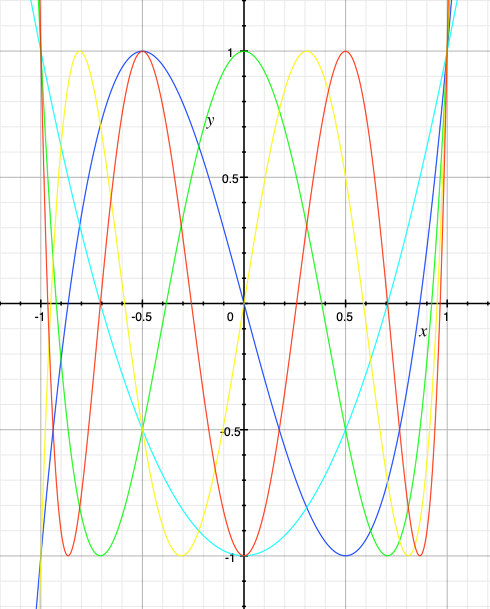
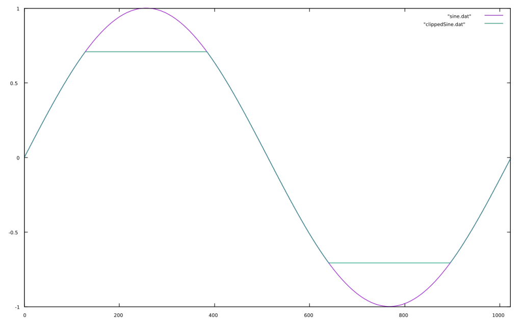
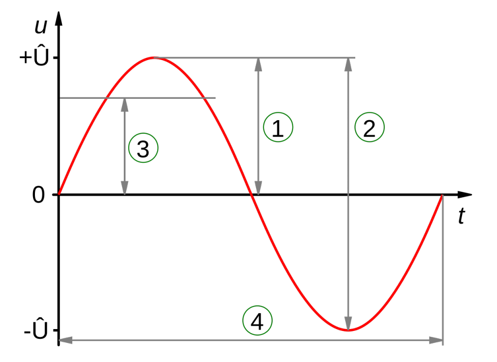
Wavefolding is a process which was originally used in the Buchla 259 complex waveform generator, a module from the Buchla 200 electronic music box and later in Serge synthesizers. It is a waveshaping function which “folds” back any input signal which exceeds a threshold. Usually there are positive and negative thresholds, so that both sides of the signal are folded. It is easiest to show this graphically.

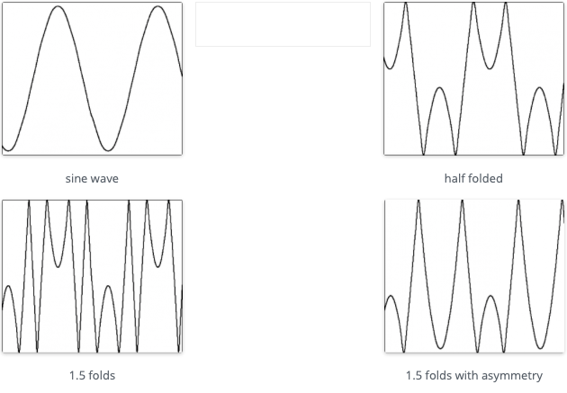
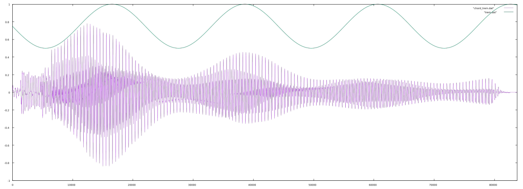
You can see how the sine wave is reversed on the top and bottom of the waveform and that this fold is reversed again in the 1.5x example when reaching the opposite threshold. The asymmetrical example is synthesized by adding a negative constant to the signal so that the negative threshold is reached before the positive one.

Wavefolding adds many new harmonics to any oscillator. This was a powerful technique on analog synthesizers as rich sounds could be created with just a handful of opamps and diodes.

Implementation

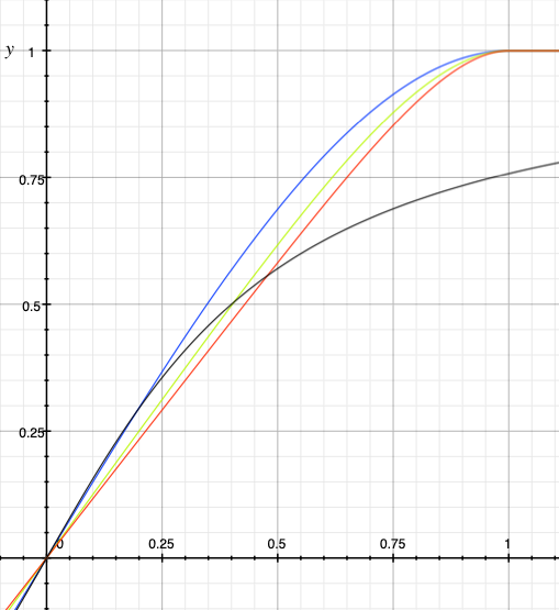
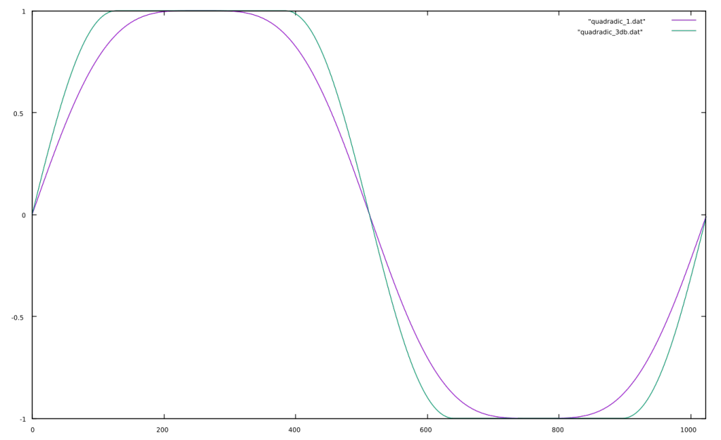
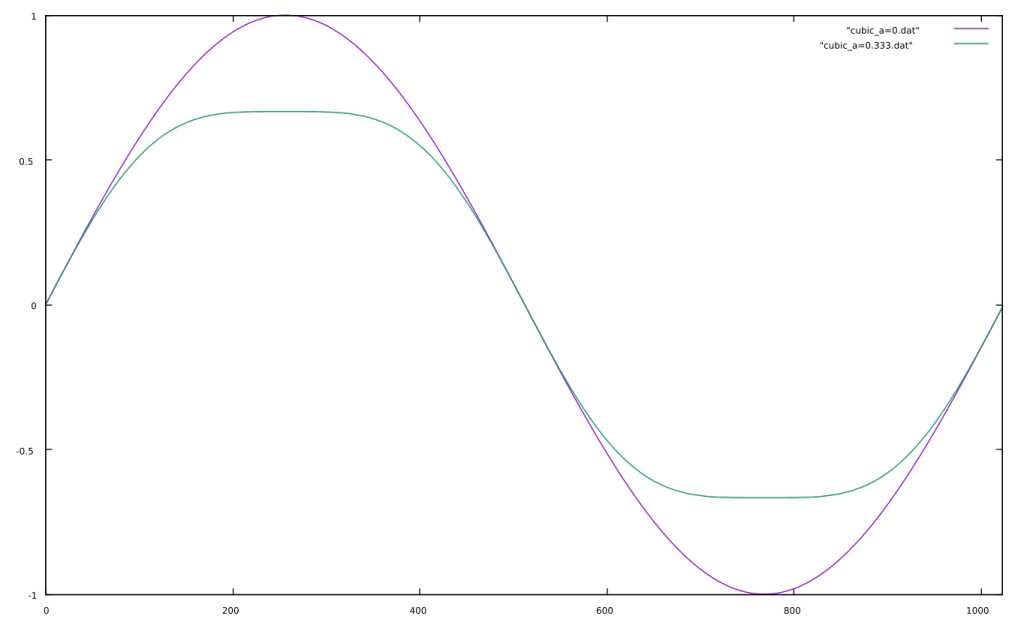
Wavefolding can be implemented by using a transfer function which reverses the signal at the positive and negative limits (-1 and 1), and again at -3, 3, -5, 5 and so on. The slope of this function should always be 1 or -1 (reversal). It is essentially a triangle wave. Here is a triangle wave approximated with it’s first 4 harmonics.

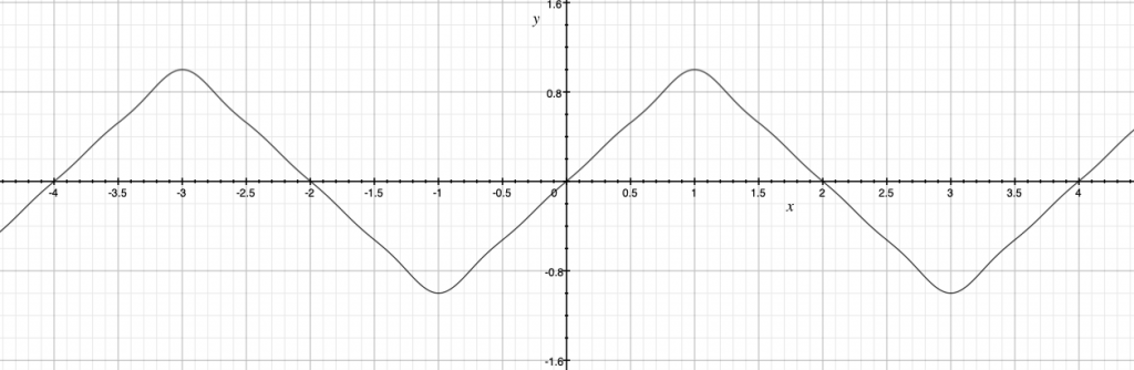
The incoming signal provides an index into the x axis, and the y axis is the output of the wavefolder. This can be implemented with a single cycle wavetable and a wrap function, or we can compute this directly from the modified triangle equation, sending the signal into x. As the signal is amplified beyond a gain of 1.0, wavefolding will start.

y_(x) = cos(.5\pi x) - \frac{1}{9} cos(1.5\pi x) + \frac{1}{25} cos(2.5\pi x) - \frac{1}{49} cos(3.5\pi x)

Here is some example C code which uses the direct synthesis method.

WaveFolder(float *input, float *output, long samples, float gain, float offset) 
{
  int sample;
  float pi = 3.141592653589793;

  // iterate through the samples in the block
  for(sample = 0; sample<samples; sample++) 
  {
    // scale the input signal by gain and add offset
    ingain = (gain * *(input+sample)) + offset;

     *(output+sample) = cos(0.5 * pi * ingain)
        - 1.0/9.0 * cos(1.5 * pi * ingain)
        + 1.0/25.0 * cos(2.5 * pi * ingain)
        - 1.0/49.0 * cos(3.5 * pi * ingain);
  }
}

The chebyshev polynomials are often used in synthesis to create harmonics from sinusoidal components. Five of the polynomials (degree 2 to 6) are plotted below:

degree 2 (light blue): y = 2x^2 - 1
degree3 (blue): y = 4x^3 - 3x
degree 4 (green): y = 8x^4 - 8x^2 + 1
degree 5 (yellow): y = 16x^5 - 20x^3 + 5x
degree 6 (red): y = 32x^6 - 48x^4 + 18x^2 - 1

These transfer functions are used for input signals within the range of -1 to 1, as the output of these functions rapidly increase beyond that. The gain on the input signal should be limited to 1.0. Because of the curved reversals in the chebyshev polynomials, they can be used as smooth wavefolders. As the input signal increases, the output quickly goes to the maximum value and wraps back. This smoothed wavefolding creates higher harmonics based on the original harmonics.

Furthermore, the chebyshev polynomials have an interesting effect on sine waves. When the sine wave is at a low level, the degree 3 polynomial will reproduce the sine wave, as the sine wave increases in volume, the 3rd harmonic will appear, and at full volume, the fundamental will disappear.

degree	harmonic transformation
2	0 – 2
3	1 – 3
4	0 – 2 – 4
5	1 – 3 – 5
6	0 – 2 – 4 – 6

One should note that if these are applied to harmonically rich waveforms or samples, every harmonic in the source signal will be multiplied. In this context, these waveshapers will create harmonic distortion and sound much like a distorted amplifier. Also, the even polynomials contain a DC component (harmonic 0). For practical use it may be necessary to remove the DC offset with a high pass filter.

When working with sine waves, the chebyshev waveshapers can be very effectively used for direct harmonic synthesis. They can also be used to replace the sine wave oscillators in additive synthesis or frequency modulation to extend those synthesis techniques.

In our section on amplitude, saturation using a cubic polynomial was shown. Alternatively polynomials of larger degree than 3 can be used. Consider the following:

y = -0.25x^5 + 1.25x

y = -0.16666x^7 + 1.16666x

The advantage of these higher degree functions is that the signal remains undistorted at larger amplitudes, and also that the gain (the slope of the saturation function) is closer to one. The disadvantage is that distortion appears more quickly when the signal reaches the saturation point.

From the plot above, the atan saturation is shown to be less linear at lower signal values. On the other hand, it goes much more slowly into saturation. For this reason, many find it to sound “warmer” than the polynomial functions.

These saturation functions are more generally known as transfer functions, or and in synthesis they are known as waveshapers. Waveshapers can be used to distort a waveform in musical ways. For instance, brass synthesis often uses a saturation waveshaper, as it makes the tone brighter when it gets louder.

Any arbitrary shape can be used in a waveshaping transfer function, and certain early digital synthesizers (Buchla 400, Buchla Touché) did just this. Discontinuous functions have been used to emulate certain fuzz pedals, or to create decimation effects (aka bitcrushing). In the next few sections we will look at a few of the types of waveshaping.

An ADSR (attack, decay, sustain, release) envelope is used to shape a note. Typically it is used to control the gain of the note, but can also be used to control amount of brightness, bass, distortion, tremolo, vibrato, or anything else that varies over the course of a note.

There are shorter and longer variations of an ADSR. The AR envelope is often used for percussive sounds. The ASR envelope is used when there is no transient at the start of a note. The DADSR envelope has a delay stage at the beginning, and is used for parameters that don’t begin immediately at the start of a note (vibrato typically begins a little after the start of the note). There can be envelopes with more stages, and many hardware synths have envelopes of 8 or more stages.

Implementation

To implement an ADSR envelope, one has to keep track it’s state. Then the envelope can do the appropriate thing for the state.

• Attack: during this state the envelope level will rise from 0.0 to 1.0 over the attack time. The envelope enters this state when the note starts. When the level reaches 1.0, the state will switch to decay.
• Decay: during this state the envelope level will drop from 1.0 to the sustain level over the decay time. When the envelope reaches the sustain level, the state will switch to sustain.
• Sustain: during this state the envelope level will be the sustain level. The envelope will stay in this state until the note ends (the key is lifted).
• Release: during this state the envelope level will drop from it’s current level to 0.0 over the release time. The envelope enters this state when the note stops (this can be during the attack, decay or sustain state).
• Off: This state is entered from the release state when the envelope level reaches 0.0. During this state, the envelope level stays at 0.0.

The code for an envelope which responds to MIDI velocity (1 to 127, note on, 0 is note off) could look like this. Notice what conditions cause the envelope to change from one state to another. Also notice that release can be entered from any state. This code should be improved in order to avoid divide by zero errors.

enum envState {
    kAttack,
    kDecay,
    kSustain,
    kRelease,
    kOff
};

long state = kOff;
float increment;
float envelopeLevel;
float samplerate = 44100;


float ADSR(float MIDIvelocity, float attacktime, float decaytime, float sustainlevel, float releasetime)
{
    switch(state)
    {
    case kOff:
        envelopeLevel = 0.0;
        if(MIDIvelocity > 0)
        {
            increment = (1.0 - envelopeLevel)/(attacktime * samplerate);
            state = kAttack;
        }
        break;
    case kAttack:
        if(envelopeLevel >= 1.0)
        {
            increment = (sustainLevel - envelopeLevel)/(decaytime * samplerate);
            state = kDecay;
        }
        break;
    case kDecay:
        if(envelopeLevel <= sustainlevel)
        {
            increment = 0.0;
            state = kSustain;
        }
    case kRelease:
        if(envelopeLevel <= 0.0)
        {
            envelopeLevel = 0.0;
            state = kOff;
        }
    }
    envelopeLevel = envelopeLevel + increment;
    if(MIDIvelocity = 0 && (state != kOff || state != kRelease)
    {
        increment = envelopeLevel/(releasetime * samplerate);
        state = kRelease;
    }
    // use MIDI velocity to change volume of envelope
    return(envelopeLevel * MIDIvelocity/127.0);  
}

Tremolo

In DSP, tremolo (not to be confused with vibrato) is a periodic amplitude variation of a signal. Most often, it appears in the form of a sine wave that subtracts from the amplitude of the signal, though technically any waveform could be used. “Classic” tremolo can be charactarized as having two parts: speed and depth which are the frequency of the sine wave (modulator) and the degree to which it modifies the signal its being applied to (the modulators amplitude). It is, essentially, a very slow amplitude modulation.

Technique

What needs to happen is to create a new signal such that if the depth of the tremolo is 0.5, the signal we multiply to the carrier oscillates between 1 and 0.5. If the depth is 0.25, then it must oscillate between 1 and 0.75, and so on. The equation we follow is:

S_{m} = 1 - d \bigg( \frac{S_{sin}}{2} + 0.5 \bigg)

Where:

S_m is the modulator (the signal that makes the tremolo effect)

S_sine is a sinewave input (oscillating between -1 and +1)

d is the depth of the tremolo between 0 and 1

This assumes that the frequency of the tremolo signal, S_sine, is set when generating that signal.

Implementation

For the input signal (signal we want tremolo on), let’s use a guitar chord:

[Listen]

For a tremolo with a depth of 0.5 and a frequency of 2Hz, we get the following:

When we multiply the input and the tremolo together, we get:

In this plot, the tremolo signal and the output are superimposed to show the relationship.

[Listen]

Autopan

An autopan effect can be created with a slight modification of our tremolo effect. The input signal will be sent to both left and right output, with gain controls on each. To make the signal appear in the center, the gain will be 0.5 for both outputs. To appear on the left, the gain will be 1.0 on the left output and 0.0 on the right output. As the left gain and right gain add up to 1.0, the right gain can be calculated as 1.0 – left gain. By using a sine wave (or other low frequency oscillator) for the left gain, an autopan effect is created. Simple C code for this effect is below.

// the samplerate in Hz
sampleRate = 44100;
// the frequency of autopan - once every 2 seconds
frequency = 0.5;
// initial phase
phase = 0.0;

void Autopan(float *input, float *outputL, float *outputR, float frequency, long samples)
{
    long sample;
    float leftgain, rightgain;
    // calculate for each sample in a block
    for(sample = 0; sample < samples; sample++)
    {
        // get the phase increment for this sample
        phaseIncrement = frequency/sampleRate;

        // calculate the gain factors
        leftgain = (sin(phase * 6.283185307179586) + 1.0) * 0.5;
        rightgain = 1.0 - leftgain;

        // calculate the output for this sample
        *(outputL+sample) = *(input+sample) * leftgain; 
        *(outputR+sample) = *(input+sample) * rightgain; 

        // increment the phase
        phase = phase + phaseIncrement;
        if(phase >= 1.0)
            phase = phase - 1.0;
    }
}

Envelope Follower

An envelope follower is used to detect signal level. This signal level can then be used in dynamics processing: gating, compression, expansion, automatic gain control, etc. Typically a combination of rectification and filtering is used to create an envelope from an audio signal.

Mean Detection

One can use the mean of a signal to follow the envelope. Essentially, a buffer is allocated and filled with samples from the signal after rectification. Then the average of the buffer is taken to be the envelope. Naturally, the larger the buffer the smoother the output but more delayed (in time) the result.

int envPosition;
int envArraySize = 64;
float envArrayTotal;
float envArray[envArraySize];

float EFGetMean(float sample) 
{   
  // wrap the index pointer   
  if(envPosition >= envArraySize)     
    envPosition = 0;  
  if(envPosition < 0)
    envPosition = 0;   
  // FIRST: rectify the input  
  if(sample < 0.0)  
    sample = -1.0 * sample;   
  // SECOND: add to array to calculate mean   
  envArrayTotal = envArrayTotal - envArray[envPosition] + sample;      
  envArray[envPosition] = sample;   
  envPosition++;   
  // THIRD: mean is total/arraysize    
  return(envArrayTotal/(float)envArraySize); 
}

All:

Zoomed:

RMS Detection

One can also calculate the RMS amplitude in an envelope follower. Similar to using the mean, the RMS method also uses a buffer, the size of which determines the smoothness and responsiveness of the envelope follower.

int envPosition;
int envArraySize = 64;
float envArrayTotal;
float envArray[envArraySize];

float EFGetRMS(float sample) 
{ 
  float square, mean;  
  // wrap the index pointer   
  if(envPosition >= envArraySize)     
    envPosition = 0;  
  if(envPosition < 0)
    envPosition = 0;   
  // FIRST: square the new sample   
  // square range 0.0 to 1.0   
  square = sample * sample;      
  // SECOND: add to array to calculate mean   
  envArrayTotal = envArrayTotal - envArray[envPosition] + square;      
  envArray[envPosition] = square;   
  envPosition++;   
  // THIRD: mean is total/arraysize    
  mean = envArrayTotal/(float)envArraySize; 
  // FOURTH: RMS is square root of mean    
  return(sqrt(mean)); 
} 

All:

Zoomed:

Attack-Release Envelope Follower

The attack-release method does not use a buffer but instead takes a moving weighted average of the peak amplitude and the sample. Here, though, one must pass the samplerate which, in part, governs the responsiveness of the follower.

float EFGetPeakAttackRelase(float attackF, float releaseF, float sample) 
{  
  float attackMultiplier;  
  float releaseMultiplier;   
  // rectify  if(sample < 0.0)  
    sample = -sample;   
  // filter   
  attackMultiplier = exp((-6.283185 * attackF)/samplerate);     
  releaseMultiplier = exp((-6.283185 * releaseF)/samplerate);    
  if(sample > peak)  
    peak = attackMultiplier * (peak - sample) + sample;  
  else  
    peak = releaseMultiplier * (peak - sample) + sample;    
  return(peak); 
}

All:

Zoomed:

Envelope Followers Compared Aurally

Plotted below are three envelope followers: mean with a window of 16, RMS with a window of 16, and attack-release with time at 1ms (attack) and 200ms (release). To test the envelope followers, we can pass noise through our resulting envelope. Here are the three enveloped plotted below.

Compression is a very common and useful signal processing device. By setting an amplitude threshold and a ratio, the dynamic range of a signal can be compressed into a smaller range. In audio, this is useful when a sound might push the boundaries of a DAC or when mixing to enable more control over the track in terms of its amplitude. The common attributes of a compressor are given below:

Parameter	Description
Threshold	The level at which the compressor “kicks in”.
Ratio	TThe ratio of compression. For example, 2:1 compression means that for every unit of amplitude the signal exceeds the threshold, it is diminished by a factor of two.
Attack Time	The time it takes for the compressor to reach full compression. This is useful since it avoids creating amplitude artifacts with quickly changing signals
Release Time	Same as the above but for the time it takes the compressor to return to normal; i.e. no amplitude correction
Makeup Gain	The amount of gain to apply post-compression.
RMS Size	In an RMS compressor, the RMS size is often controllable.

The basic form of a compressor is an envelope follower whose output is passed to a function that checks whether or not the amplitude has exceeded the threshold and if so, by what amount. If the amplitude exceeds the threshold, an amplitude correction is multiplied to the signal using the ratio. After compression is applied, the makeup gain is applied and the signal is sent out. In the below example of an RMS compressor, the smoothing of the attack and release are accomplished with the use of a single-pole low pass filter. Without smoothing, amplitude artifacts would be introduced into the output. It is also assumed that one has an RMS function (`getRMS()) elsewhere.

float gain = 0; // initial value 
float diff = 0; // initial value  

RMSCompressor(float *input, float *output, long samples, float threshold = 0.707, float ratio = 2, float attTime = 0.003, float relTime = 0.03, float makeupGain = 0, int rmsSize = 64) 
{   
  // the coefficient for the attack   
  double attCoeff = 1 - exp(-1/(SAMPLERATE*attTime)); 
  // the coefficient for the release   
  double relCoeff = 1 - exp(-1/(SAMPLERATE*relTime)); 
  // get the ratio factor   
  float ratioFac = 1 - (1/ratio); 
  // a buffer for RMS calculations   
  float *rmsBuff[] = new float[rmsSize]; 

  for(sample = 0; sample < samplesPerBlock; sample++) 
  {
    // get the RMS amplitude     
    rmsAmp = getRMS(*(input+sample), rmsBuff); 
    diff = *(input+sample) - threshold; // get the difference 
    if(diff>1.0) diff = 1.0;    
    if(diff>0) 
    {       
      // the signal exceeds the threshold. 
      // Apply compression using a single-pole low pass 
      // to smooth out the attack.       
      gain = gain + (attCoeff*((1-(diff*ratioFac))-gain));     
    } 
    else
    {       
      // else we need to return to normal
      // a gain of 1 (no correction)       
      gain = gain + (relCoeff*(1-gain));     
    }
    *(output+sample) = gain * *(input+sample) * (1+makeupGain); 
  }
}

When applied to a signal, the dynamic range is compressed. The image below is an overlay of an original signal (purple) and a compressed version (green) sampled at 44.1kHz. Note how the amplitude peaks on the compressed version are lower than the original. The following image shows the amplitude correction applied to the signal to create the compressed version. The compressor used was 5:1 with a threshold of 0.5, an attack time of 0.003, a release time of 0.03, and a makeup gain of 0.

More extreme compression with the threshold set to 0.2 and the ratio as 50:1.

And the same again but with the attack time set to 0.03 and the release time to 0.3.

The Limiter

A limiter can be thought of as a type of compressor with certain settings such that it only makes itself known at the extreme ends of amplitude and in a very high degree. This is usually intended for peak reduction, but also for leveling a mix in mastering. Typical parameters might be a threshold of 0.9 linear amplitude, a ratio of 40, and very fast attack and release.

What if the peak amplitude exceeds 1?

If the peak amplitude exceeds 1, the result is distortion of the signal in the form of clipping. This can damage certain hardware and is best avoided.

If the level above 1 is known, one can simply multiply the signal by 1 minus that value.

More likely, however, whether or not the amplitude will exceed 1 is unknown. In this case there are several options: hard clipping. soft clipping, limiters, or compressors.

Hard Clipping

Hard clipping is done by limiting the maximum and minimum sample values. When a signal exceeds the limit, a hard edge is created that creates high frequency harmonics (distortion).

HardClip(float *input, float *output, long samples, float limit) 
{
  // iterate through the samples in the block
  for(int sample = 0; sample<samples; sample++) 
  {
    // check if it's greater than limit or less than -limit
    if(*(input+sample) > limit)
      *(output+sample) = limit;
    else if(*(input+sample) < -1.0 * limit)
      *(output+sample) = -1.0 * limit;
    else
      *(output+sample) = *(input+sample);
  }
}

In this image, the purple line is a sine that is unclipped with a maximum amplitude of 1. The green line is a sine that is clipped at -3 dB (approx. 0.707 linear amplitude). Notice the hard edge at the clipping limit.

Soft Clipping

Soft clipping is another method of clipping that softens the edges of the clipped boundary using non-linear functions. This can be done several ways; most often, however, you’ll see the use of the tangent function or quadratic functions.

Cubic Equation Soft Clipping

By calculating the coefficients beforehand, creating a soft clipper with the cubic equation can be relatively fast. This method, however, does not allow scaling via a gain coefficient and thus acts to shield the output from being driven too hard.

y = -0.5x^3 + 0x^2 + 1.5x + 0

Simplified

y = -0.5x^3 + 1.5x $$y = -0.5x^3 + 1.5x$$

QuadraticSoftClip(float *input, float *output, long samples, float limit, float gain) 
{
  int samplenumber = 0;
  float a = -0.5f;
  float b = 0.0;
  float c = 1.5f;
  float d = 0.0;
  float ingain;
 
  // iterate through the samples in the block
  for(sample = 0; sample<samples; sample++) 
  {
    ingain = gain * *(input+sample); // get the input
 
    // if it's greater than 1, hard clip
    if(ingain > 1.0)
      *(output+sample) = 1.0;
    // if it's less than -1, hardclip
    else if(ingain < -1.0)
      *(output+sample) = -1.0;
    // else, do the softclipping
    else
      *(output+sample) = a * ingain * ingain * ingain
        + b * ingain * ingain
        + c * ingain
        + d;
  }
}

Here is a plot of a sine wave run through this function when the input gain is 1 (0dB, purple) and 1.412 (+3dB, green). When this function is ran, you can see the distortion occur as the steepening of the angle as the waveform ascends and descends. Notice, however, that when the input gain is above unity, the function prevents it from going above 1.

Cubic Soft Clipping Simplified

y = x - \bigg( \alpha \cdot x^3 \bigg )

$$y = x - \bigg( \alpha \cdot x^3 \bigg )$$

In this function, alpha is the scaling coefficient and can vary between 0 and the limit. It is typically 1/3 and produces a clipped level of about -3dB. When the scaling coefficient is 0, the signal is passed unaffected (no clipping, no distortion) but as alpha is increased, the waveform is clipped softly.

Tangent Function Soft Clipping

y = \frac{2}{\pi} \text{ } arctan(\alpha \cdot x)

$$y = \frac{2}{\pi} \text{ } arctan(\alpha \cdot x)$$

Notice that when alpha >> 10, the function approaches infinite clipping distortion; i.e. approaches a square wave with soft edges.

Thoughts

Although both of these methods can produce soft clipping, the cubic functions are generally more efficient since trigonometric calculations must be performed on every sample in the tangent function.

By cascading multiple softclippers, one can crudely approximate analog distortion.

Amplitude

In digital sound, amplitude is a measurement of the strength of a signal, usually between 0 and 1 (linearly) or between -infinity and 0 in decibels (dB). Colloquially, amplitude can be thought of as the volume of a sound (not loudness), also called sound pressure level (SPL). Changing the amplitude of a sound is akin to turning a volume knob up or down on a car stereo.

The decibel (dB)

Since our ear responds logarithmically to the amplitude of sound, amplitude (SPL) is most typically measured in decibels. A decibel is a unit of measurement that expresses the ratio of one quantity to another; that is, in order to express something in decibels, we need a reference value. In the case of SPL, our reference is 0dB_spl = 20 microPascals (considered to be the threshold of human hearing) Note the ratio in the logarithm of the equation for calculating the SPL of sound:

L_{p} = 20 \log_{10} \bigg(\frac{p_{rms}}{p_{ref}}\bigg) \text{ dB}

In audio, we most often speak of decibels as if it is a relative quantity. For instance, if we consider 0dB the loudest sound in digital audio with an amplitude of 1.0, we obtain the following linear amplitudes.

dB	linear amplitude
0	1
-3	0.707945
-6	0.501187
-9	0.354813
-12	0.251188

Peak v. RMS

When measuring the amplitude of a signal, either the peak or root mean square (RMS) amplitude can be used. (Notice in the equation above that the numerator of the fraction is p_rms which is the sound pressure level in root mean square (RMS) amplitude.)

In the graphic above, each number is the following:

1. Peak amplitude (Û)
2. Peak-to-peak amplitude (2Û)
3. RMS amplitude (Û/√2)
4. Period (not a measurement of amplitude)

In digital audio, we often use both peak and RMS amplitude. Peak-to-peak amplitude is almost never used since signals are typically centered around 0 (if you signal is not, there is a DC component that can be removed LINK TO RELEVANT FILE LATER).

What if the peak amplitude exceeds 1?

If the peak amplitude exceeds 1, the result is distortion of the signal in the form of clipping. This can damage certain hardware and is best avoided. If the level above 1 is known, one can simply multiply the signal by 1 minus that value. More likely, however, whether or not the amplitude will exceed 1 is unknown. In this case there are several options: hard clipping. soft clipping, limiters, or compressors.

With a frequency tunable allpass filter, it is simple to create both low pass and high pass filters. As the first order allpass has a phase shift of π at the nyquist frequency and a phase shift of zero at 0 Hz, it can be added to the input to create a lowpass filter. To maintain the same amplitude at 0 Hz, the output is multiplied by 1/2. The following C code show this slight modification to the first order allpass filter.

double in1 = 0; // delayed sample
double out = 0; // keep track of the last output

folp(float *input, float *output, long samples, float cutoff) 
{
    double tf = tan(PI * (cutoff/SAMPLERATE)); // tangent frequency
    double c = (tf - 1.0)/(tf + 1.0); // coefficient

    for(int i = 0; i < samples; i++) 
    {
        double sample = *(input+i);
        out = (c*sample) + in1 - (c * out); // get the output
        in1 = sample; // remember it
        *(output+i) = (sample+out)*0.5; 
       // add and scale to get lowpass
  }
}

At the cutoff frequency, there will be a phase shift of π/2 (90 degrees) at the output of the allpass. When we add the input to the allpass output, we will have a combined phase shift of (π/4) and a gain equal to half the hypotenuse of 1 and 1 – or 0.70710678. This gain is approximately -3 dB. This graph shows the gain and phase shift of a low pass filter set to 1000Hz.

A first order highpass is almost identical to the lowpass except the allpass output is subtracted from the input.

double in1 = 0; // delayed sample
double out = 0; // keep track of the last output

fohp(float *input, float *output, long samples, float cutoff) 
{
    double tf = tan(PI * (cutoff/SAMPLERATE)); // tangent frequency
    double c = (tf - 1.0)/(tf + 1.0); // coefficient

    for(int i = 0; i < samples; i++) 
    {
        double sample = *(input+i);
        out = (c*sample) + in1 - (c * out); // get the output
        in1 = sample; // remember it
        *(output+i) = (sample-out)*0.5; 
       // add and scale to get highpass
  }
}