An allpass filter passes a signal with the same gain response for all frequencies. Without affecting the gain response, an allpass filter changes the frequency phase. This response can be graphed from -π to π over the audio frequency range.
The allpass filter can be used as a building block in filter construction, using phase cancellation to form standard lowpass, highpass, bandpass, and notch filters; as well as typical effects such as chorusing, flanging, and phasing.
First Order
A first order allpass is called this because it uses a one sample delay in its implementation.
y[n] = c(x[n]) + x[n-1] - c(y[n-1])
The coefficient c is calculated from the tangent of the frequency, tf, fc is the cutoff frequency, and sr is the sampling rate:
You might notice that a frequency of 0 will result in a coefficient of -1 and a frequency at half the sample rate (the Nyquist frequency) will result in an error, as tan(π/2) is ∞. Because of this, the frequency should be limited to less than half the sample rate. The coefficient approaches 1 as the frequency approaches the Nyquist frequency.
The first order allpass filter has a phase shift of 0 at 0 Hz, π at the Nyquist frequency and π/2 at the cutoff frequency. The following C code can implement this filter. Note that double floating point variables are used for feedback terms. This is because mathematical error can build up in a feedback network, and using doubles will minimize this error.
double in1 = 0; // delayed sample
double out = 0; // keep track of the last output

foap(float *input, float *output, long samples, float cutoff)
{
    double tf = tan(PI * (cutoff/SAMPLERATE)); // tangent frequency
    double c = (tf - 1.0)/(tf + 1.0); // coefficient
    for(int i = 0; i < samples; i++)
    {
        float sample = *(input+i);
        out = (c*sample) + in1 - (c * out);
        in1 = sample; // remember input
        *(output+i) = out; // output
    }
}
In this section two simple filters are presented. Both use feedback of the previous output samples in the calculation of new samples. When samples are averaged, high frequencies are diminished. When samples are differentiated, low frequencies are diminished.
One Pole Low Pass
The first is a one-pole low pass filter. The new output sample can clearly be seen as a crossfade between the input and the previous output.
out = in * (1 - c) + out1 * c;
out1 = out;
The amount of in/out “crossfade” is the filter coefficient c. You can get an intuitive feeling for the filter coefficient c by observing that each output sample is an mix between the previous output and the input. As the coefficient c is increased, this mix contains mostly previous output, and this averaging between the mix of previous samples and the current sample smooths out the waveform – it reduces the high frequencies.
As the coefficient c is lowered, the filtering is reduced, and when c is 0.0, the input is copied to the output unfiltered.
This type of filter is also known as a exponentially weighted moving average filter. You can find the derivation for the exact coefficient c for a given filter frequency elsewhere, but the following approximation is often used.
c = exp(-2 * PI * frequency/samplingRate);
You can obtain a high-pass by subtracting the low-pass output from the input.
hpout = new - out;
Simple Band Pass Filter
The following filter was used in Max Mathew’s filter opcode in Music IV and a derivation is used in Barry Vercoe’s reson opcode in Csound.
out = in + c1 * out1 - c2 * out2;
out2 = out1;
out1 = out;
This filter is somewhat similar to the moving average filter above, and when c2 is zero, it is very similar. When c2 increases, the output 2 samples previous is removed from the moving average. This diminishes the low frequency component and gives the entire filter a bandpass characteristic. In Max Mathew’s implementation, the two coefficients c1 and c2 are calculated for any given bandwidth and frequency.
c1 = 2.0 * exp(-1.0 * PI * bandwidth/samplingRate) * cos(2 * PI * frequency/samplingRate);
c2 = exp(-2 * PI * bandwidth/samplingRate);
Coefficient calculation and sound processing
In these two filters there is one section of code to calculate the coefficients from a given frequency and bandwidth (or more detailed parameters) and another section for filtering the audio (using those coefficients and saving the internal state in one or more state variables). It’s typical for the coefficient calculation to be more CPU intensive than the filter calculation. This is because coefficient calculation involves trigonometric functions. For many instances the coefficients can be precalculated for the range of frequencies and bandwidths used.
One can also add sine waves together (additive synthesis) to approximate the basic forms presented earlier in this section. Individual sine waves of appropriate frequencies and amplitudes (with matching phases) can be used or one can use a lookup method and fill the table with the sum of the waves. The latter method is shown here.
Sawtooth and Ramp
The sawtooth has perhaps the most simple formula: given a harmonic series of sine waves, multiply each by the reciprocal of their harmonic number and sum. For instance, the first harmonic is multiplied by 1/1, the second harmonic, is multiplied by 1/2, the third harmonic is multiplied by 1/3, and so on. In other words:
where k is the number of harmonics and sin(2πfkt) is a sine wave.
float table[1024];
int harmonics = 10; // 10 harmonics
float amp = 1.0; // amplitude
float max = 0; // for normalization

// clear the table
for(i=0; i < tableSize; i++) '
   table[i] = 0.0;

// fill the table
for(k=1; k <= harmonics; k++)
{
    // for each harmonic, go through and add it to the table
    for(i=0; i < tableSize; i++)
    {
        float samp;
        samp = (i*k)/tableSize; // get the increment
        samp = samp * 2PI; // scale the frequency
        table[i] = table[i] + (sin(samp) * 1/harmonic); // add it
        if (table[i] > max)
            max = table[i]; // remember it if it's the largest value we've encountere
    }
}

// normalize
for(i=0; i < tableSize; i++)
   table[i] = table[i]/max; // scale
The following is an animation of the process. N is the number of harmonics used to construct the wave. Notice that as N increases, the result is increasingly sharp and similar to an algebraically constructed sawtooth.
Ramp
The ramp is created by simply inverting the phase of the sine wave used in the sawtooth:
float table[1024];
int harmonics = 10; // 10 harmonics
float amp = 1.0; // amplitude
float max = 0; // for normalization

for(i=0; i<tableSize; i++)
    table[i] = 0.0;
// fill the table
for(k=1; k <= harmonics; k++)
{
   // if the harmonic is odd, go through and add it to the table
   if (k & 1 == 1)
   {
      for(i=0; i < tableSize; i++)
      {
          float samp;
          samp = (i*k)/tableSize; // get the increment
          samp = samp * 2PI; // scale the frequency
          table[i] = table[i] + (sin(samp) * 1/harmonic); // add it
          if (table[i] > max)
              max = table[i]; // remember it if it's the largest value we've encountered
      }
   }
}

// normalize
for(i=0; i < tableSize; i++)
    table[i] = table[i]/max; // scale
Notice that in the same way as the sawtooth, when we increase the number of harmonics of the square wave we more closely resemble an algebraically constructed one.
Triangle
The triangle wave, like the square wave, uses only odd harmonics but the phase of every other harmonic is inverted (multiplied by -1 or phase change by π). The amplitude of the harmonics, however, is the reciprocal of the square of their mode number. This means that the first harmonic is multiplied by 1/1<sup>2</sup>, the third harmonic is multiplied by 1/3<sup>2</sup>, the fifth by 1/5<sup>2</sup>, etc.
float table[1024];
int harmonics = 10; // 10 harmonics
float amp = 1.0; // amplitude
float max = 0; // for normalization
boolean invertPhase = false; // boolean to invert the phase

for(i=0; i<tableSize; i++)
    table[i] = 0.0;

//fill the table
for(k=1; k <= harmonics; k++)
{
    // if the harmonic is odd, go through and add it to the table
    if (k & 1 == 1)
    {
        for(i=0; i < tableSize; i++)
        {
            float samp;
            samp = (i*k)/tableSize; // get the increment
            samp = samp * 2PI;
            // scale the frequency
            table[i] = table[i] + (sin(samp) * 1/(harmonic**2));
            // add it
            if (invertPhase)
            {
                table[i] = -1 * table[i]; // invert the phase
                invertPhase = false; // don't invert next time
            }
            else
                invertPhase = true; // invert the next time
            if (table[i] > max)
                max = table[i]; // remember it if it's the largest value we've encountered for normalization
         }
     }
}

// normalize
for(i=0; i < tableSize; i++)
    table[i] = table[i]/max; // scale
Notice that in the same way as the sawtooth, when we increase the number of harmonics of the triangle wave we more closely resemble an algebraically constructed one.
Addition using individual Sinewaves
In the same way we can populate a table to create a waveform, one can also generate and add the same sine tones individually and sum them in the output. The technique is to essentially calculate the relative amplitudes using the same formulas as before, put them in a table, and read from them during playback.
float frequency = 440; // fundamental in Hz
int harms = 10; // number of harmonics
float phase;
float harmonicAmp[harms+1]; // a table to keep the amplitudes in

// define a function to calculate the amplitudes
double sawtoothAmp(int harm)
{
    return(1.0/(double)harm);
}

// populate the table of amplitudes
for(i=1; i <= harms; i++) {
  harmonicAmp[i] = sawtoothAmp(i);
}

// calculate a block
for(sample = 0; sample < samples; sample++)
{
    // the phase increment is linearly
    // related to sample rate
    phase += (frequency * 6.28318531)/samplerate;
    sawtooth = 0.0;
    for(harm = 1; harm <= harms; harm++)
        sawtooth += sin(phase * harm) * harmonicAmp[harm];
    output[sample] = sawtooth;
}
Using this technique, one could also address the amplitude of each harmonic individually after the waveform has been created. This could allow one to blend waveforms in time.
Complex sinusoids are two-dimensional signals whose value at any instant can be specified by a complex number; that is, a number with real part and an imaginary part. These two parts are in what is known as phase quadrature with one another; i.e. the imaginary part is pi/2 radians out of phase with the real part (1/4 of a cycle). That is why the components of the complex signal are sometimes known as in-phase and quadrature phase.
A complex sinusoid is defined by the following mathematical representations:
Cartesian Form: x(t) \triangleq Acos(\omega t + \phi) + jAsin(\omega t + \phi)
Polar Form: (t) = Ae^{j(\omega t + \phi)}
where A is amplitude, ω is the angular frequency in radians per second (the frequency in Hertz scaled by 2π; 2πf), ϕ is the initial phase offset in radians, and t is time in seconds. The cosine portion of the sinusoid is the real component and the sine portion is the imaginary (phase quadrature) component. (In engineering, the variable j is typically denoted to mean the square root of negative 1, whereas pure math often uses the variable i to mean the same thing).
Projection
Recall the Pythagorean Identity: cos^2(\phi) + sin^2(\phi) = 1
Reconfiguring the Cartesian form of a complex sinusoid with this in mind, we get: |x(t)| \triangleq \sqrt{re^2\{x(t)\} + im\{x(t)\}} \equiv A
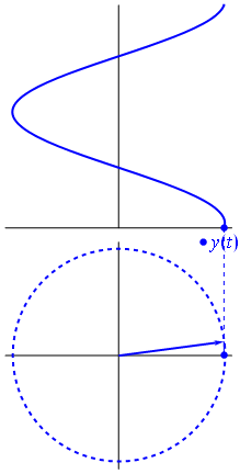
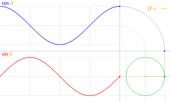
In other words, a complex sinusoid has a constant complex magnitude (A). Since this is true, the projection of a complex signal (in complex form) onto the complex plane must lie on a circle; i.e. the radius (magnitude) remains the same while the angle changes). Recall the animation in the beginning of this section:
This animation shows the counter-clockwise motion of the real (cosine) component of the complex sinusoid projected onto the complex plane. We can also project the complex phasor onto orthogonal axes:
The green circle in the bottom right corner is the unit circle in the complex plane. We can rewrite the trigonometric form of the equation into polar form: cos\theta + jsin\theta = re^{j\theta}
where j is the square root of negative 1, r is the length (or magnitude), θ is the angle in radians, and e is Euler’s number.
Relabeling a sine wave:
Advantages
Representing a sinewave in complex form has several distinct advantages:
Instantaneous Frequency: f = \omega + \frac{d}{dt}\phi(t)
Instantaneous Phase: \angle x(t) = \omega t + \phi
Instantaneous Magnitude (Amplitude): A = \sqrt{re^2\{x(t)\} + im\{x(t)\}}
Using complex sinusoid generation in an oscillator
This method of calculation can be used for a fairly efficient sine and cosine wave generator. The only CPU intensive calculation is the calculation of the complex phase factor. If using a limited set of frequencies, the complex phase could be pre-calculated in a table.
double cosZ, sinZ;

SinComplex(float freq, float *output, long samplesPerBlock)
{
	long sample;
	float freqAngle, angleReal, angleImag;

	freqAngle = twoPi * freq;
        // calculate the phose angle for given frequency
	angleReal = cos(freqAngle);
	angleImag = sin(freqAngle);
	for(sample = 0; sample<samplesPerBlock; sample++)
        {
            // complex multiply by phase angle for sin output
            *(output+sample) = angleReal * sinZ - angleImag * cosZ;
            // complex multiply by phase angle for cos output
            cosZ = angleReal * cosZ + angleImag * sinZ;
            sinZ = *(output+sample);
            // correction for accumulated computation inaccuracies
            if(sinZ < -1.0) sinZ = -1.0;
            if(sinZ > 1.0f) sinZ = 1.0f;
        }
}
When we use phase truncation on a phasor whose frequency is low relative the tablesize and sampling rate, consecutive samples may not change. To counter this, we can use different methods of interpolation to more accurately represent the waveforms when the periods of the phasor are very small compared to the size of the table.
It is essentially the ratio between the period of the phasor and size of the table…
Linear Interpolation
Linear interpolation involves using the fractional part of the calculated phase to calculate the “distance” between the two points on which we lie. If, for instance, our calculated index is 32.76, we would need to look at both indexes 32 and 33. We would then take their respective values, `t[32]` and `t[33]`, calculate the difference between the latter index and the earlier, multiply by the fractional part, then add it to the index as we would in phase truncation:
 // calculate the fractional part
frac = index - int(index);

// get the difference and wrap the index (can also use a modulo)
while(index > tablesize)
    index = index - tablesize;

if (index == tablesize-1)
    diff = t[0] - t[index]; // wrap
else
    diff = t[index+1] - t[index]; // no need to wrap

// get the interpolated output
out = t[index] + (diff * frac);
where `t` is the table filled with the sine wave and `index` is the calculated index with a phasor multiplied by the size of the table minus 1.
Hermite (Cubic) Interpolation
A more accurate interpolation technique is the Hermite or cubic method. What this method essentially does is to find the coefficients a, b, c, and d for the third degree polynomial f(x) and its derivative, f'(x), at x = 0 and x = 1.
\begin{aligned}& f(x) = ax^3 + bx^2 + cx + d \\ & f'(x) = 3ax^2 + 2bx + c \end{aligned}
Calculating the Coefficients
Given four points, (x0, y0), (x1, y1), (x2, y2), (x3, y3), we can calculate the coefficients with the following:
\begin{aligned} & a = -\frac{y_{0}}{2} + \frac{3y_{1}}{2} - \frac{3y_{2}}{2} + \frac{y_{3}}{2} \\ & b = y_{0} - \frac{5y_{1}}{2} + 2y_{2} - \frac{y_{3}}{2} \\ & c = -\frac{y_{0}}{2} + \frac{y_{2}}{2} \\ & d = y_{1} \end{aligned} This is called the Catmull-Rom spline.
Calculating these coefficients and plugging them into the third degree polynomial (the first equation) gives us the cubic interpolative values between x = 0 and x = 1.
Putting it Together
Given an index i, we need to get the indices i-1, i, i+1, and i+2 to use them in our cubic interpolator.
float cubicInterpolator(float idx, float *table)
{
    long trunc = (long) idx; // truncate the index but don't overwrite
    float frac = idx - trunc; // get the fractional part

    // get the indices
    int x0 = wrap(trunc-1, tableSize-1);
    int x1 = wrap(trunc, tableSize-1);
    int x2 = wrap(trunc+1, tableSize-1);
    int x3 = wrap(trunc+2, tableSize-1);

    // calculate the coefficients
    float a = -0.5*table[x0] + 1.5*table[x1] - 1.5*table[x2] + 0.5*table[x3];
    float b = table[x0] - 2.5*table[x1] + 2.0*table[x2] - 0.5*table[x3];
    float c = -0.5*table[x0] + 0.5*table[x2];
    float d = table[x1];

    return (a*(frac*frac*frac) + b*(frac*frac) + c*frac + d);
}
Phase Truncation, Linear Interpolation, and Cubic Interpolation Compared
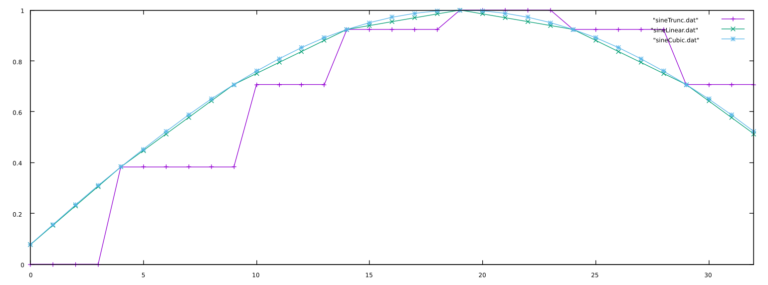
If we push this to an extreme to show the differences, this plot shows samples 32 to 64 of the same 100Hz sine wave lookup sampled at 8kHz using either phase truncation (purple), linear interpolation (green), or cubic interpolation (blue) from a tablesize of 16:
Listen
Listen to each of the different interpolation methods below. Be particularly aware of the differences at extremely high and low frequencies.
sine sweep with phase truncationsine sweep with 2 point linear interpolationsine sweep with 4 point cubic interpolation
Often it is much more efficient to create a waveform using a lookup table as opposed to calculating the output directly. This is most often the case with the most acoustically simple waveform, the sine wave. One can calculate a sine wave from a phasor by multiplying the phasor by 2π, the number of radians in a circle, such that the phasor now extends from 0 to 2π. That value is then used in a sine operation such that the final equation looks like this:
f(x) = sin(\phi2\pi)
or:
sin(phasor(f)*2.0*PI);
where `PI` is the value of π and `f` is the frequency in Hz of the waveform. This, however, means that the sine of the phasor is calculated for every sample. On the other hand, if we populate a table with a single cycle of a precomputed sine wave, all that needs to be done is to index into the table at the rate of the frequency of the sine wave desired.
static double 2PI = 3.14159 * 2.0; // two pi
int tablesize = 1024; // size of the table
double *sinetable = malloc(tablesize); // allocate a table

// fill the table
for(int i = 0; i < tablesize; i++)
    sinetable[i] = sin((2PI*i)/tablesize);
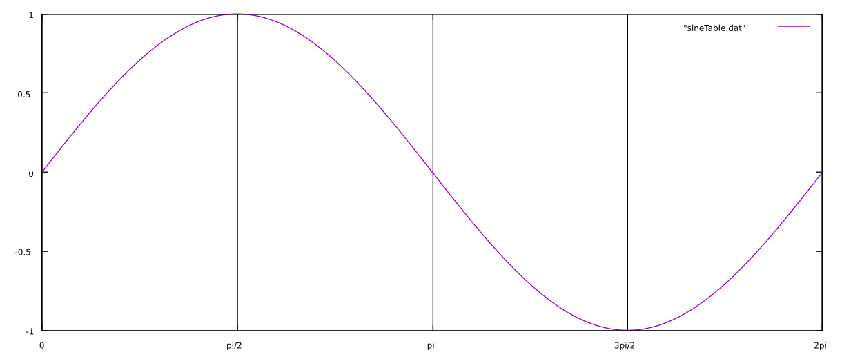
Using a tablesize of 1024, the table looks like this:
To index into this table, we need to use integers. If we take a phasor at some desired frequency, we can take the output and multiply it by the size of the table minus one (since in most languages we start counting from 0) and cut off the fractional part to obtain an index:
i = \lfloor \phi * s \rfloor
where s is the size of the table and phi is the value of the phasor from 0 to 1. In code:
index = int(phasor(f)*tablesize);
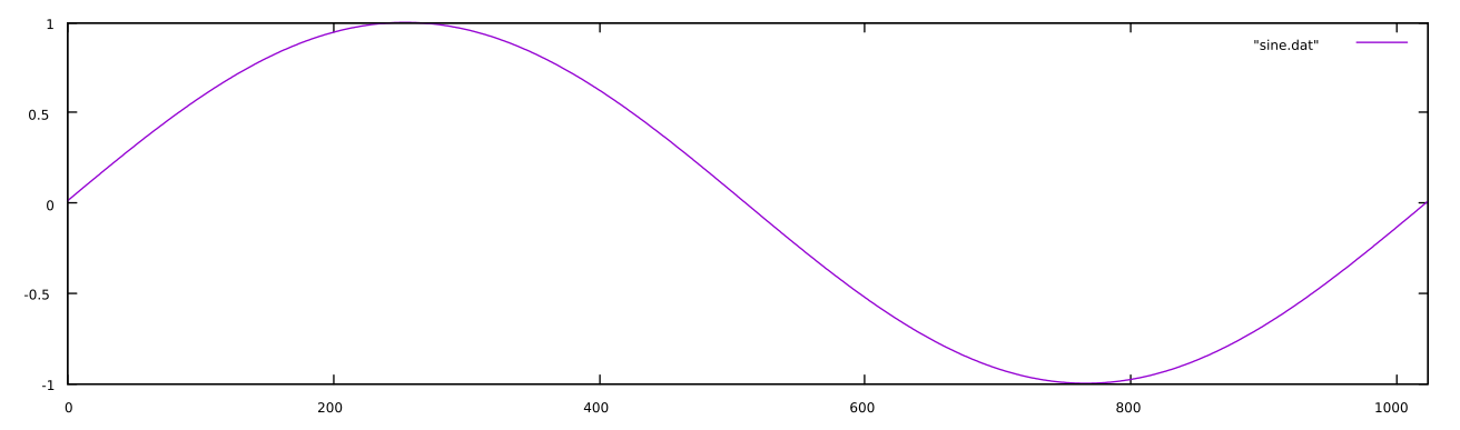
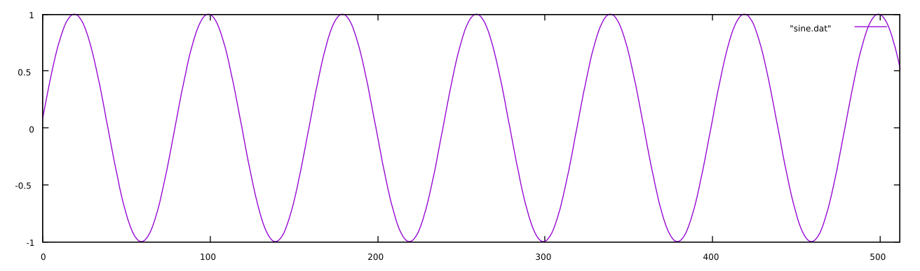
This method of simply removing the fractional part of the phase is called phase truncation. We can then use this output to index into the table and get the correct value for the sine wave. Below are the first 512 samples of a 100Hz phasor indexing into a wavetable of size 1024 at an 8kHz samplerate:
Two other simple waveforms, the square and triangle, can also be created with the phasor as input. As with the simple ramp and sawtooth, these are more useful as low frequency modulating oscillators than they are as audio oscillators.
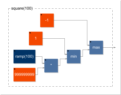
Square
The square wave is just that: a waveform that resembles a square. It is a special case of the pulse wave, which we will see later, where the duty cycle (the ratio between the high and low points) is 50%. It can be created algebraically or via logic operations.
Using algebra
Caveat: this method resembled the engineering technique BFI more than a clean algebraic method.
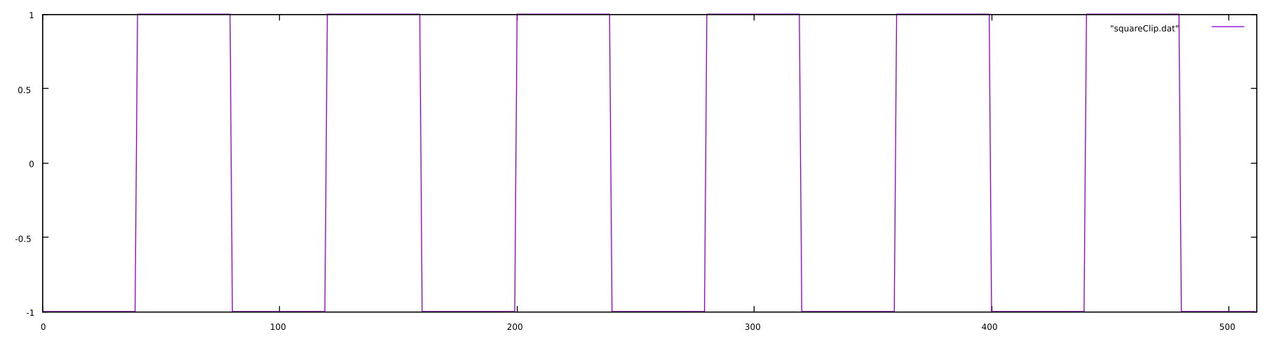
One method of this is to create a ramp or sawtooth, multiply it by some very high number, and clip it at -1 and +1: `(ramp*9999999).clip(-1,1)`.
// make a clip function

float clip(float n, float lower, float upper)
{
    if(n<lower) return lower;
    else if (n>upper) return upper;
    else return n;
}

void Osc::Square(float *frequency, float *output, long samplesPerBlock)
{
    long sample;
    float rampPhase;
    // calculate for each sample in a block
    for(sample = 0; sample<samplesPerBlock; sample++)
    {
        // get the phase increment for this sample
        phaseIncrement = *(frequency + sample)/sampleRate;
        // make a ramp (-1 to +1)
        rampPhase = (phase*2.0) - 1.0;
        // get the output for this sample
        *(output+sample) = clip(ramp*9999999999, -1.0, 1.0);
        // increment the phase
        phase = phase + phaseIncrement;
    }
}
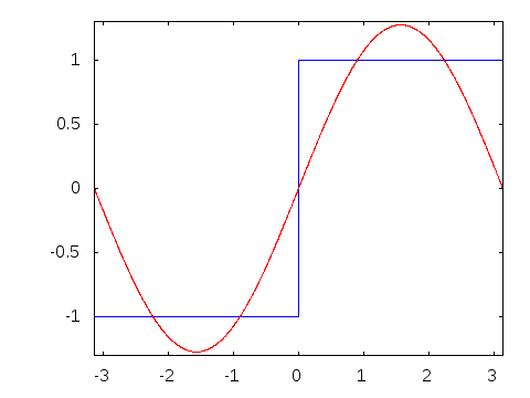
This method is very closely related to the sign method of creating the square wave in which the sign of a sinusoid is used to get either -1 or +1:
x(t) = sgn(sin fT)
Counting samples
One can also count the number of samples in a period. That is, if we know our sample rate is 1000Hz and we want a square wave at a frequency of 50Hz, we know that a complete period of the square wave will be 1000/50 or `samplerate/frequency`. This means that a 50Hz square wave (or any waveform, for that matter) at a 1000Hz sample rate is going to have a period of 20 samples. Since we know that a square wave’s duty cycle is 50%, we know that the wave will be +1 for 10 samples, then -1 for 10 samples.
NOTE: This is related to BLIP and BLEP
Using logic
Perhaps a bit cleaner is to use logical operations on a phasor:
void Osc::Square(float *frequency, float *output, long samplesPerBlock)
{
    long sample;
    // calculate for each sample in a block
    for(sample = 0; sample<samplesPerBlock; sample++)
    {
        // get the phase increment for this sample
        phaseIncrement = *(frequency + sample)/sampleRate;

        // calculate the output for this sample
        if(phase <= 0) *(output+sample) = -1.0;
        else *(output+sample) = 1.0;
        // increment the phase
        phase = phase + phaseIncrement;
    }
}
Combining a ramp and a sawtooth
One can also sum a ramp and a sawtooth, offset in phase by 1/2 of a cycle to create a square. We will see this method in the future when we use it to create pulses of different lengths in pulse width modulation.
float phaseRamp, phaseSaw;

void Osc::SquarePMW(float frequency, float width, float *output, long samplesPerBlock)
{
    // width varies between 0.0 and 1.0, width is 0.5 for square
    long sample;
    float ramp, saw, square;
    // calculate for each sample in a block
    for(sample = 0; sample<samplesPerBlock; sample++)
    {
        phasePerSample = frequency/sampleRate;
        ramp = (phaseRamp * 2.0) - 1.0;
        saw = -1.0 * ((phaseSaw * 2.0) - 1.0);
        square = ramp + saw;
        // ((width - 0.5) * 2) needs to be added to
        // the sum to make waveform symmetrical around 0
        square = square + ((width - 0.5) * 2.0);
        *(output+sample) = square;

        phaseRamp = phaseRamp + phasePerSample;
        if(phaseRamp > 1.0) phaseRamp = phaseRamp - 1.0;
        if(phaseRamp <= 0.0) phaseRamp = phaseRamp + 1.0;
        phaseSaw = phaseRamp + width;
        if(phaseSaw > 1.0) phaseSaw = phaseSaw - 1.0;
    }
}
Whatever method is used, the result looks something like this:
Triangle
The triangle wave is another of the basic waveforms. It forms a triangle, centered about 0, that linearly ascends from -1 to +1, then from +1 to -1.
Using algebra
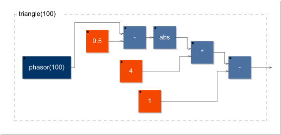
If the input is a phasor, we can create a triangle wave using absolute value and some multiplication:
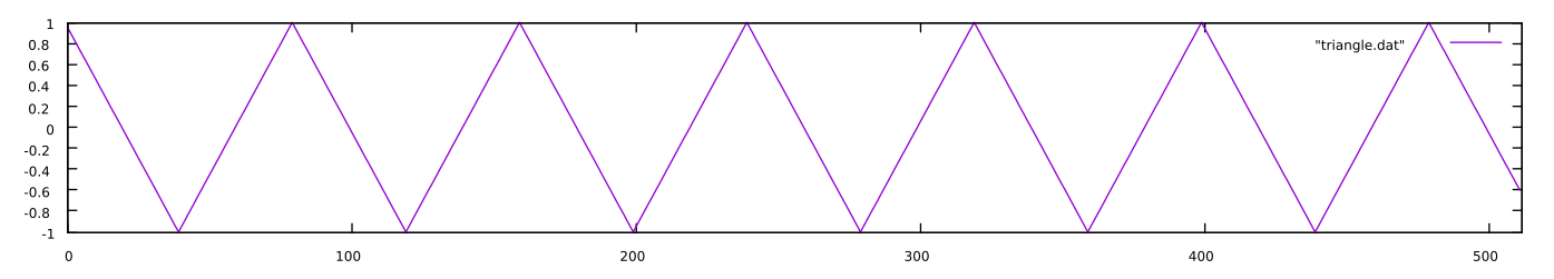
`triangle = (abs(phasor-0.5)*4)-1;`
This method creates a triangle wave that begins it’s cycle at the crest of the waveform. Here are the first 512 samples of a 100Hz triangle wave sampled at 8kHz.
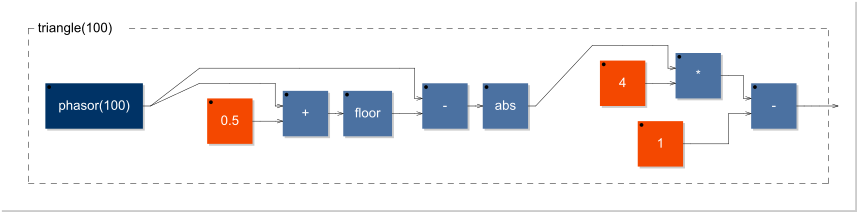
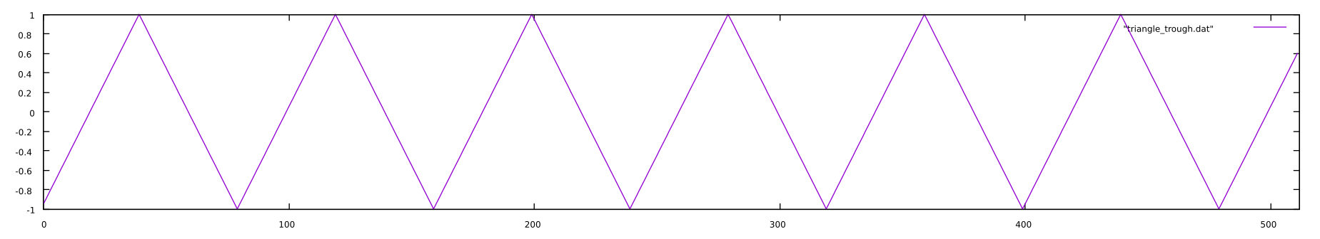
We can also use a slightly different method but using the floor function, or truncation, in addition to absolute value, where truncation removes the decimal portion of a floating point value (essentially rounding _down_ to the nearest integer).
The ramp wave and a sawtooth wave are mirror images of one another. The ramp ascends linearly from -1 to +1 while the sawtooth descends linearly from +1 to -1. The methods here will produce a non-bandlimited waveforms and will produce audible aliasing. This aliasing makes this type of oscillator less desirable for audio. However, they can be useful as a source of modulation – as a low frequency oscillator (LFO).
Ramp
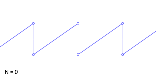
A ramp wave is essentially a phasor that goes from -1 to +1.
Using the phasor as the starting point, it is fairly straightforward to create a ramp algebraically:
That is, take the phasor, multiply it by two and subtract one. This results in a ramp that ascends from -1 to +1. Or: `(phasor*2)-1`. This results in the following waveform, the first 512 samples of a 100Hz ramp at a samplerate of 8kHz:
Listen
Notice that since this oscillator is not bandlimited one can hear the aliasing very clearly, especially when changing the frequency. [Click here to listen.](src/ramp/rampPlay.html)
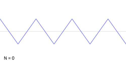
Sawtooth
A sawtooth wave is ramp that _descends_ from +1 to -1.
Using algebra
Using the phasor as the starting point, it is fairly straightforward to create a ramp algebraically:
That is, take the phasor, multiply it by two and subtract one. This results in a sawtooth wave that descends from +1 to -1. Or: `(phasor * -2) + 1`. This results in the following waveform, the first 512 samples of a 100Hz sawtooth at a samplerate of 8kHz:
Listen
Notice that since this oscillator is not bandlimited one can hear the aliasing very clearly, especially when changing the frequency. It sounds identical to the ramp.
The phasor is perhaps the most simple and fundamental of oscillators. It takes the shape of a sawtooth wave but has two important differences:
1. It ascends from 0 to 1, as opposed from -1 to +1.
2. It is _not_ bandlimited (in discrete time this matters).
x{phasor}(t) = \frac{t}{p} \text{mod } 1
where p is the period in Hertz and t is time.
sampleRate = 128;    // the samplerate in Hz
freq = 1;            // the frequency in Hz
phasePerSecond = freq;  // the change in phase per unit of time;
                        // i.e. the frequency when time is seconds
phasePerSample = freq/sampleRate;   // the amount of change in phase per
                                    // sample for a given frequency at a
                                    // given samplerate
Osc::Osc()
{
    phase = 0.0;
    phasePerSample = 0.0;
}

void Osc::Phasor(float frequency, float *output, long samplesPerBlock)
{
    long sample;
    // calculate for each sample in a block
    for(sample = 0; sample<samplesPerBlock; sample++)
    {
        phasePerSample = frequency/sampleRate; // get the phase increment for this sample
        *(output+sample) = phase; // calculate the output for this sample
        phase = phase + phasePerSample; // increment the phase
    }
}
Important here is the relationship between `phasePerSample` and `freq`: they are, in fact, representations of the same thing. With frequency, we give the total number of rotations (oscillations) in a second while phase per sample is the rate of change at the sampling period. If we want to give an oscillator a frequency, we will need to calculate the change in phase per sample; i.e. `phasePerSample`.
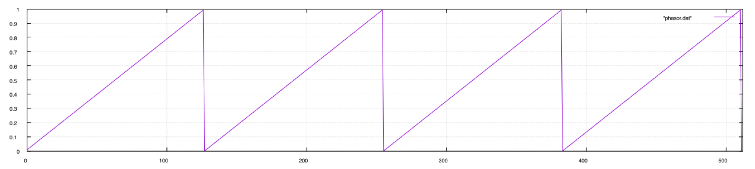
Using a samplerate of 128Hz, the first 512 samples of a 1Hz phasor are plotted below:
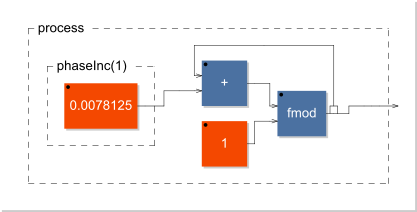
Notice how the waveform ascends from 0 to 1 as noted above. This makes it extraordinarily useful in waveshaping, indexing into tables, etc. As a simplified block diagram, the phasor looks like this:
`phaseInc(1)` is the phase increment for a 1Hz signal at a 128Hz samplerate. 1/128 = 0.0078125.