Interpolation

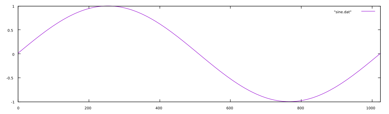
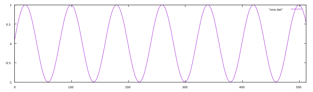
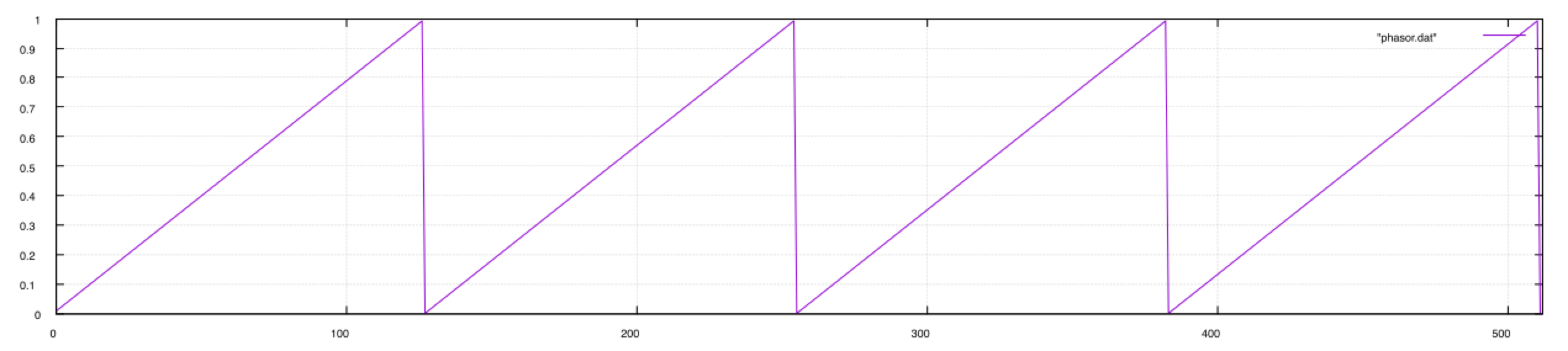
When we use phase truncation on a phasor whose frequency is low relative the tablesize and sampling rate, consecutive samples may not change. To counter this, we can use different methods of interpolation to more accurately represent the waveforms when the periods of the phasor are very small compared to the size of the table.

It is essentially the ratio between the period of the phasor and size of the table…

Linear Interpolation

Linear interpolation involves using the fractional part of the calculated phase to calculate the “distance” between the two points on which we lie. If, for instance, our calculated index is 32.76, we would need to look at both indexes 32 and 33. We would then take their respective values, `t[32]` and `t[33]`, calculate the difference between the latter index and the earlier, multiply by the fractional part, then add it to the index as we would in phase truncation:

 // calculate the fractional part
frac = index - int(index);

// get the difference and wrap the index (can also use a modulo)
while(index > tablesize)
    index = index - tablesize;

if (index == tablesize-1) 
    diff = t[0] - t[index]; // wrap
else
    diff = t[index+1] - t[index]; // no need to wrap

// get the interpolated output
out = t[index] + (diff * frac);

where `t` is the table filled with the sine wave and `index` is the calculated index with a phasor multiplied by the size of the table minus 1.

Hermite (Cubic) Interpolation

A more accurate interpolation technique is the Hermite or cubic method. What this method essentially does is to find the coefficients a, b, c, and d for the third degree polynomial f(x) and its derivative, f'(x), at x = 0 and x = 1.

Calculating the Coefficients

Given four points, (x0, y0), (x1, y1), (x2, y2), (x3, y3), we can calculate the coefficients with the following:

\begin{aligned} & a = -\frac{y_{0}}{2} + \frac{3y_{1}}{2} - \frac{3y_{2}}{2} + \frac{y_{3}}{2} \\ & b = y_{0} - \frac{5y_{1}}{2} + 2y_{2} - \frac{y_{3}}{2} \\ & c = -\frac{y_{0}}{2} + \frac{y_{2}}{2} \\ & d = y_{1} \end{aligned}
This is called the Catmull-Rom spline.

Calculating these coefficients and plugging them into the third degree polynomial (the first equation) gives us the cubic interpolative values between x = 0 and x = 1.

Putting it Together

Given an index i, we need to get the indices i-1, i, i+1, and i+2 to use them in our cubic interpolator.

float cubicInterpolator(float idx, float *table)
{
    long trunc = (long) idx; // truncate the index but don't overwrite
    float frac = idx - trunc; // get the fractional part

    // get the indices
    int x0 = wrap(trunc-1, tableSize-1);
    int x1 = wrap(trunc, tableSize-1);
    int x2 = wrap(trunc+1, tableSize-1);
    int x3 = wrap(trunc+2, tableSize-1);

    // calculate the coefficients
    float a = -0.5*table[x0] + 1.5*table[x1] - 1.5*table[x2] + 0.5*table[x3];
    float b = table[x0] - 2.5*table[x1] + 2.0*table[x2] - 0.5*table[x3];
    float c = -0.5*table[x0] + 0.5*table[x2];
    float d = table[x1];

    return (a*(frac*frac*frac) + b*(frac*frac) + c*frac + d);
}

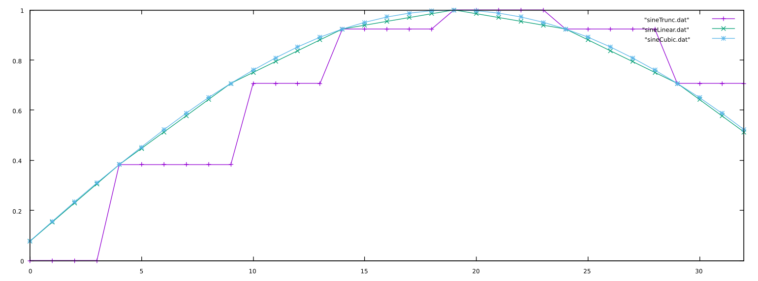
Phase Truncation, Linear Interpolation, and Cubic Interpolation Compared

If we push this to an extreme to show the differences, this plot shows samples 32 to 64 of the same 100Hz sine wave lookup sampled at 8kHz using either phase truncation (purple), linear interpolation (green), or cubic interpolation (blue) from a tablesize of 16:

Listen

Listen to each of the different interpolation methods below. Be particularly aware of the differences at extremely high and low frequencies.

Table Lookup Oscillators

Often it is much more efficient to create a waveform using a lookup table as opposed to calculating the output directly. This is most often the case with the most acoustically simple waveform, the sine wave. One can calculate a sine wave from a phasor by multiplying the phasor by 2π, the number of radians in a circle, such that the phasor now extends from 0 to 2π. That value is then used in a sine operation such that the final equation looks like this:

f(x) = sin(\phi2\pi)

or:

sin(phasor(f)*2.0*PI);

where `PI` is the value of π and `f` is the frequency in Hz of the waveform. This, however, means that the sine of the phasor is calculated for every sample. On the other hand, if we populate a table with a single cycle of a precomputed sine wave, all that needs to be done is to index into the table at the rate of the frequency of the sine wave desired.

static double 2PI = 3.14159 * 2.0; // two pi
int tablesize = 1024; // size of the table
double *sinetable = malloc(tablesize); // allocate a table

// fill the table
for(int i = 0; i < tablesize; i++)
    sinetable[i] = sin((2PI*i)/tablesize);

Using a tablesize of 1024, the table looks like this:

To index into this table, we need to use integers. If we take a phasor at some desired frequency, we can take the output and multiply it by the size of the table minus one (since in most languages we start counting from 0) and cut off the fractional part to obtain an index:

i = \lfloor \phi * s \rfloor

where s is the size of the table and phi is the value of the phasor from 0 to 1. In code:

index = int(phasor(f)*tablesize);

This method of simply removing the fractional part of the phase is called phase truncation. We can then use this output to index into the table and get the correct value for the sine wave. Below are the first 512 samples of a 100Hz phasor indexing into a wavetable of size 1024 at an 8kHz samplerate:

Square and Triangle

Two other simple waveforms, the square and triangle, can also be created with the phasor as input. As with the simple ramp and sawtooth, these are more useful as low frequency modulating oscillators than they are as audio oscillators.

Square

The square wave is just that: a waveform that resembles a square. It is a special case of the pulse wave, which we will see later, where the duty cycle (the ratio between the high and low points) is 50%. It can be created algebraically or via logic operations.

Using algebra

Caveat: this method resembled the engineering technique BFI more than a clean algebraic method.

One method of this is to create a ramp or sawtooth, multiply it by some very high number, and clip it at -1 and +1: `(ramp*9999999).clip(-1,1)`.

// make a clip function

float clip(float n, float lower, float upper)
{
    if(n<lower) return lower;
    else if (n>upper) return upper;
    else return n;
}

void Osc::Square(float *frequency, float *output, long samplesPerBlock)
{
    long sample;
    float rampPhase;
    // calculate for each sample in a block
    for(sample = 0; sample<samplesPerBlock; sample++)
    {
        // get the phase increment for this sample
        phaseIncrement = *(frequency + sample)/sampleRate; 
        // make a ramp (-1 to +1)
        rampPhase = (phase*2.0) - 1.0; 
        // get the output for this sample
        *(output+sample) = clip(ramp*9999999999, -1.0, 1.0); 
        // increment the phase
        phase = phase + phaseIncrement; 
    }
}

This method is very closely related to the sign method of creating the square wave in which the sign of a sinusoid is used to get either -1 or +1:

Counting samples

One can also count the number of samples in a period. That is, if we know our sample rate is 1000Hz and we want a square wave at a frequency of 50Hz, we know that a complete period of the square wave will be 1000/50 or `samplerate/frequency`. This means that a 50Hz square wave (or any waveform, for that matter) at a 1000Hz sample rate is going to have a period of 20 samples. Since we know that a square wave’s duty cycle is 50%, we know that the wave will be +1 for 10 samples, then -1 for 10 samples.

NOTE: This is related to BLIP and BLEP

Using logic

Perhaps a bit cleaner is to use logical operations on a phasor:

void Osc::Square(float *frequency, float *output, long samplesPerBlock)
{
    long sample;
    // calculate for each sample in a block
    for(sample = 0; sample<samplesPerBlock; sample++)
    {
        // get the phase increment for this sample
        phaseIncrement = *(frequency + sample)/sampleRate; 

        // calculate the output for this sample
        if(phase <= 0) *(output+sample) = -1.0;
        else *(output+sample) = 1.0;
        // increment the phase
        phase = phase + phaseIncrement; 
    }
}

Combining a ramp and a sawtooth

One can also sum a ramp and a sawtooth, offset in phase by 1/2 of a cycle to create a square. We will see this method in the future when we use it to create pulses of different lengths in pulse width modulation.

float phaseRamp, phaseSaw;

void Osc::SquarePMW(float frequency, float width, float *output, long samplesPerBlock)
{
    // width varies between 0.0 and 1.0, width is 0.5 for square
    long sample;
    float ramp, saw, square;
    // calculate for each sample in a block
    for(sample = 0; sample<samplesPerBlock; sample++)
    {
        phasePerSample = frequency/sampleRate;
        ramp = (phaseRamp * 2.0) - 1.0;
        saw = -1.0 * ((phaseSaw * 2.0) - 1.0);
        square = ramp + saw;
        // ((width - 0.5) * 2) needs to be added to
        // the sum to make waveform symmetrical around 0
        square = square + ((width - 0.5) * 2.0);
        *(output+sample) = square;

        phaseRamp = phaseRamp + phasePerSample; 
        if(phaseRamp > 1.0) phaseRamp = phaseRamp - 1.0;
        if(phaseRamp <= 0.0) phaseRamp = phaseRamp + 1.0;  
        phaseSaw = phaseRamp + width;
        if(phaseSaw > 1.0) phaseSaw = phaseSaw - 1.0;     
    }
} 

Whatever method is used, the result looks something like this:

Triangle

The triangle wave is another of the basic waveforms. It forms a triangle, centered about 0, that linearly ascends from -1 to +1, then from +1 to -1.

Using algebra

If the input is a phasor, we can create a triangle wave using absolute value and some multiplication:

`triangle = (abs(phasor-0.5)*4)-1;`

This method creates a triangle wave that begins it’s cycle at the crest of the waveform. Here are the first 512 samples of a 100Hz triangle wave sampled at 8kHz.

We can also use a slightly different method but using the floor function, or truncation, in addition to absolute value, where truncation removes the decimal portion of a floating point value (essentially rounding _down_ to the nearest integer).

where _p_ is the period and _t_ is time in seconds.

`triangle(f) = (4 * abs(phasor(f) – trunc(phasor(f) + 0.5))) – 1`

This method, as opposed to the one above, creates a triangle wave that begins its cycle at the trough:

When implemented either way, the result sounds like this:

Ramp and Sawtooth

The ramp wave and a sawtooth wave are mirror images of one another. The ramp ascends linearly from -1 to +1 while the sawtooth descends linearly from +1 to -1. The methods here will produce a non-bandlimited waveforms and will produce audible aliasing. This aliasing makes this type of oscillator less desirable for audio. However, they can be useful as a source of modulation – as a low frequency oscillator (LFO).

Ramp

A ramp wave is essentially a phasor that goes from -1 to +1.

x_{ramp}(t) = 2 \bigg( \frac{t}{p} \text{mod } 1 \bigg) - 1

Using algebra

Using the phasor as the starting point, it is fairly straightforward to create a ramp algebraically:

That is, take the phasor, multiply it by two and subtract one. This results in a ramp that ascends from -1 to +1. Or: `(phasor*2)-1`. This results in the following waveform, the first 512 samples of a 100Hz ramp at a samplerate of 8kHz:

Listen

Notice that since this oscillator is not bandlimited one can hear the aliasing very clearly, especially when changing the frequency. [Click here to listen.](src/ramp/rampPlay.html)

Sawtooth

A sawtooth wave is ramp that _descends_ from +1 to -1.

Using algebra

Using the phasor as the starting point, it is fairly straightforward to create a ramp algebraically:

x_{sawtooth}(t) = -2 \bigg( \frac{t}{p} \text{mod } 1 \bigg) + 1

That is, take the phasor, multiply it by two and subtract one. This results in a sawtooth wave that descends from +1 to -1. Or: `(phasor * -2) + 1`. This results in the following waveform, the first 512 samples of a 100Hz sawtooth at a samplerate of 8kHz:

Listen

Notice that since this oscillator is not bandlimited one can hear the aliasing very clearly, especially when changing the frequency. It sounds identical to the ramp.

The Phasor

The phasor is perhaps the most simple and fundamental of oscillators. It takes the shape of a sawtooth wave but has two important differences:

1. It ascends from 0 to 1, as opposed from -1 to +1.
2. It is _not_ bandlimited (in discrete time this matters).

x{phasor}(t) = \frac{t}{p} \text{mod } 1

where p is the period in Hertz and t is time.

sampleRate = 128;    // the samplerate in Hz
freq = 1;            // the frequency in Hz
phasePerSecond = freq;  // the change in phase per unit of time; 
                        // i.e. the frequency when time is seconds
phasePerSample = freq/sampleRate;   // the amount of change in phase per 
                                    // sample for a given frequency at a 
                                    // given samplerate
Osc::Osc()
{
    phase = 0.0;
    phasePerSample = 0.0;
}

void Osc::Phasor(float frequency, float *output, long samplesPerBlock)
{
    long sample;
    // calculate for each sample in a block
    for(sample = 0; sample<samplesPerBlock; sample++)
    {
        phasePerSample = frequency/sampleRate; // get the phase increment for this sample
        *(output+sample) = phase; // calculate the output for this sample
        phase = phase + phasePerSample; // increment the phase
    }
}

Important here is the relationship between `phasePerSample` and `freq`: they are, in fact, representations of the same thing. With frequency, we give the total number of rotations (oscillations) in a second while phase per sample is the rate of change at the sampling period. If we want to give an oscillator a frequency, we will need to calculate the change in phase per sample; i.e. `phasePerSample`.

Using a samplerate of 128Hz, the first 512 samples of a 1Hz phasor are plotted below:

Notice how the waveform ascends from 0 to 1 as noted above. This makes it extraordinarily useful in waveshaping, indexing into tables, etc. As a simplified block diagram, the phasor looks like this:

`phaseInc(1)` is the phase increment for a 1Hz signal at a 128Hz samplerate. 1/128 = 0.0078125.

Oscillators

The most basic sound-generating process in digital sound is the oscillator. An oscillator creates a periodic waveform of some shape (sine, square, saw, triangle, etc) and repeats it in time. The number of times it repeats per second is its fundamental frequency. This is measured in units of Hertz (Hz) or cycles per second. The reciprocal of frequency is the period, or the number of seconds per cycle.

As a concept

Unit Circle

It is helpful to visualize a sine oscillator as a wheel and spoke.

The angle of the “spoke” is the phase at a given moment in time while the frequency are the number of rotations per second. The length (magnitude) of the spoke is the amplitude at any given point.

Phase

The phase of a waveform, often denoted with the Greek letter phi (Φ), is a means to define a specifc point on a waveform. Phase change is measured on a unit circle, that is, a circle with a radius of 1.0. As the circumference of the circle is 2πr, one rotation has 2π of phase. The unit used to measure phase is the radian.

Sampled Signals

When programming digital audio, we will be working primarily with sampled waveforms. A waveform is generated by calculating samples at a certain (and usually a fixed) rate. This is the sample rate (seconds per sample).

To convert time to a number of samples, simply multiply the time in seconds by the sample rate. For instance: an oscillator at 200 Hz has a period of 1/200 (or .005) seconds. To find the number of samples for this period with a sample rate of 44100; multiply 44100 * .005. The answer is 220.5 samples.

The micro USB port on the STMF4Discovery board is a OTG (“on the go”) USB port. This means it can function as both a slave or master USB port. To use it as a MIDI host (so we can use MIDI keyboard and fader controllers) we need a OTG adapter. Here is one from Amazon. These are typically used to attach flash drives to Android phones. The STM32Cube has an example of USB Host and Device code in the Middleware folder. However, instead of using that to develop a class-compliant MIDI host, I have simply adapted Xavier Halgand‘s USB MIDI host code to work with the current version of the STM HAL libraries. Xavier is the author of the wonderful Dekrispator synthesizer for the STM32F4Discovery board.

My MIDI framework with a basic (terrible sounding) polyphonic synthesizer can be downloaded here: f4disco-midi. You should be able to to unzip, place it in your workspace folder, and import to STM32CubeIDE.

You will see a number of things added to this project, including a struct and enum to support each synthesizer voice. Each voice represents an independent sound generator, and these can become fairly complex. Our voice will be a simple, unaliased, sawtooth oscillator with a fixed ASR gain envelope. It requires the following for each voice:

typedef struct synthVoice
{
    int active;
    int note;
    int velocity;
    float volume;
    float frequency;
    float phase;
} synthVoice;

typedef enum
{
    INACTIVE = 0,
    ATTACK,
    DECAY,
    SUSTAIN,
    RELEASE
} voiceState;

The active variable will indicate the various states that each voice can be in, these states are in the following enum. The remaining members of the synthVoice struct are synthesis parameters. Later you will see 16 synthVoices being allocated

synthVoice voice[16];

In the function main(), the USB MIDI driver is initialized, and then two functions are called in the main while loop. The function MIDIApplication() parses any MIDI received through USB, and the function USBH_Process(&hUSBHost) maintains the USB connection – it allows plugging and unplugging of USB devices.

/*## Init Host Library ################################################*/
 USBH_Init(&hUSBHost, USBH_UserProcess_callback, 0);
/*## Add Supported Class ##############################################*/
 USBH_RegisterClass(&hUSBHost, USBH_MIDI_CLASS);
/*## Start Host Process ###############################################*/
 USBH_Start(&hUSBHost);

// Initialize and start audio codec
BSP_AUDIO_OUT_Init(OUTPUT_DEVICE_HEADPHONE, 90, 48000);
BSP_AUDIO_OUT_Play((uint16_t *)codecBuffer, 128);
 /* USER CODE END 2 */
/* Infinite loop */
 /* USER CODE BEGIN WHILE */
 while (1)
 {
     HAL_Delay(1);
     /* USER CODE END WHILE */
     // MX_USB_HOST_Process();
    /* USER CODE BEGIN 3 */
    MIDI_Application();
    /* USBH_Background Process */
    USBH_Process(&hUSBHost);
 }

MIDI_Application() calls a function I wrote called ProcessMIDI(). This processes one MIDI message, identifying the byte code for the type of MIDI message, and copys the data from the message. I have implemented the parsing for “note on”, “note off” and “controller change”. Framework for other MIDI messages (status type), is included. To parse all of the types of MIDI message, you will need to refer to the MIDI Specification (easily found online).

void ProcessMIDI(midi_package_t pack)
{
	int i;
	uint8_t status;

	// Status messages that start with F, for all MIDI channels
	// None of these are implemented - though we will flash an LED
	// for the MIDI clock
	status = pack.evnt0 & 0xF0;
	if(status == 0xF0)
	{
		switch(pack.evnt0)
		{
		case 0xF0:	// Start of System Exclusive
		case 0xF1:	// MIDI Time Code Quarter Fram
		case 0xF2:	// Song Position Pointer
		case 0xF3:	// Song Select
		case 0xF4:	// Undefined
		case 0xF5:	// Undefined
		case 0xF6:	// Tune Request
		case 0xF7:	// End of System Exclusive
			status = runningStatus = 0x00;
			break;
		case 0xF8:	// Timing Clock (24 times a quarter note)
			HAL_GPIO_TogglePin(LD5_GPIO_Port, LD5_Pin); // RED LED
			break;
		case 0xF9:	// Undefined
		case 0xFA:	// Start Sequence
		case 0xFB:	// Continue Sequence
		case 0xFC:	// Pause Sequence
		case 0xFD:	// Undefined
		case 0xFE:	// Active Sensing
		case 0xFF:	// Reset all synthesizers to power up
			break;

		}
	}

// MIDI running status (same status as last message) doesn't seem to work over this USB driver
// code commented out.

//	else if((pack.evnt0 & 0x80) == 0x00)
//		status = runningStatus;
	else
		runningStatus = status = pack.evnt0 & 0xF0;



	switch(status)
	{
	case 0x80:	// Note Off
		// turn off all voices that match the note off note
		for(i = 0; i<16; i++)
		{
			if(voice[i].note == pack.evnt1)
			{
				voice[i].active = RELEASE;
				keyboard[voice[i].note] = -1;
			}
		}
		break;
	case 0x90:	// Note On
		if(pack.evnt2 == 0) // velocity 0 means note off
			// turn off all voices that match the note off note
			for(i = 0; i<16; i++)
			{
				if((voice[i].note == pack.evnt1) && (voice[i].active != INACTIVE))
				{
					voice[i].active = RELEASE;
					keyboard[voice[i].note] = -1;
				}
			}
		else
		{
			// if this key is already on, end the associated note and turn it off
			if(keyboard[pack.evnt1] != -1)
			{
				voice[keyboard[pack.evnt1]].active = RELEASE;
				keyboard[pack.evnt1] = -1;
			}
			// find an inactive voice and assign this key to it
			for(i = 0; i<16; i++)
			{
				if(voice[i].active == INACTIVE)
				{
					voice[i].active = ATTACK;
					voice[i].note = pack.evnt1;
					voice[i].velocity = pack.evnt2;
					keyboard[pack.evnt1] = i;
					break;
				}
			}
		}
		break;
	case 0xA0:	// Polyphonic Pressure
		break;
	case 0xB0:	// Control Change
		switch(pack.evnt1) // CC number
		{
		case 3 	:
			break ;	// tempo
		case 7 :
			break;	// master volume
		}
		break;
	case 0xC0:	// Program Change
		break;
	case 0xD0:	// After Touch
		break;
	case 0xE0:	// Pitch Bend
		pitchbend = pack.evnt2 * 128 + pack.evnt1;
		break;
	}
}

My implementation of ProcessMIDI() doesn’t do voice allocation (though it does look for inactive voices before assigning a new one), and isn’t doing anything with the data from CC (controller change) messages. There is lots of room for improvement, this is just intended as a starting point.

The audioBlock() audio callback function has been modified to generate up to 16 voices, each synthesizing a harsh sawtooth wave. The data set in ProcessMIDI() is being used to set the frequency of each voice, and to manage the ASR envelope in each voice. Note that when a note off is received by ProcessMIDI, the voice is not made inactive. Instead, the voice is put in the RELEASE part of the envelope, and is only made INACTIVE when the envelope reaches zero.

void audioBlock(float *input, float *output, int32_t samples)
{
    int i, v;
    float increment1, increment2;
    for(i = 0; i < samples; i += 2)
        output[i<<1] = output[(i<<1) + 1] = 0.0f;
    for(v = 0; v < 16; v++)
    {
        if(voice[v].active != INACTIVE)
         {
             voice[v].frequency = mtoinc[voice[v].note];
           for(i = 0; i < samples; i += 2)
            {
                voice[v].phase += voice[v].frequency;
              if(voice[v].phase > 1.0f)
                    voice[v].phase = voice[v].phase - 1.0f;
                output[i<<1] += ((voice[v].phase * 2.0f) - 1.0f) * voice[v].volume * 0.125f;
                output[(i<<1) + 1] = output[i<<1];
              if(voice[v].active == ATTACK)
                {
                    voice[v].volume += 0.02f;
                  if(voice[v].volume >= 1.0f)
                        voice[v].active = SUSTAIN;
                }
              else if(voice[v].active == SUSTAIN)
                    voice[v].volume = 1.0f;
              else if(voice[v].active == RELEASE)
                {
                    voice[v].volume -= 0.0002f;
                  if(voice[v].volume <= 0.0f)
                        voice[v].active = INACTIVE;
                }
            }
        }
    }
}

This code should be useful as a starting point for synthesizer creation. Those creating drum machines or effects processors will want to handle MIDI messages differently.

For this next change we will need to add some source code which has been developed to support the circuit board and the specific devices on the board. First, in the IDE, you will need to create a folder in the “Drivers” folder. Name this new folder “BSP”. Now we will copy some code into “BSP.”  When you started the IDE it should have downloaded the board and chip support code. Look for the folder STM32Cube and under that Repository:STM32Cube_FW_F4_V1.24.1. Under that you will find Drivers:BSP. This stands for board specific package. Find the folder for STM32F4-Discovery and make a copy of it in your project by dropping the folder on your “BSP” IDE folder – select “Copy…”

You now need to do the same for BSP:Components. Drag and drop “Components” on “BSP”. Finally, there is a folder with code that supports the on-board microphone. It is Middleware:ST:STM32Audio. Drag and drop “STM32Audio” on the IDE folder “Middleware:ST”. When done, your project will look like this

Once this is done, we should be able to Build the project and have no errors.

Making sound

To make sound we need to call functions to initialize the CODEC, start the CODEC and we need to periodically call functions to compute samples for the CODEC. The BSP functions in stm32f4_discovery_audio.c make the first two steps fairly simple. To initialize the CODEC call the functions:

BSP_AUDIO_OUT_Init(OUTPUT_DEVICE_HEADPHONE, 90, 48000);
BSP_AUDIO_OUT_Play((uint16_t *)codecBuffer, 128);

after  “/* USER CODE BEGIN 2 */.” We also need to a include statements on the top of main.c so that main.c can see the declarations of the functions and macros we want to use. Add:

#include "../Drivers/BSP/STM32F4-Discovery/stm32f4_discovery_audio.h"

after “/* USER CODE BEGIN Includes */.” Finally, we need to define the array “codecBuffer”. We can declare it as a global (as well as globals for the I2S serial device) after “/* USER CODE BEGIN PV */”

int16_t codecBuffer[64];    // 32 samples X 2 channels
extern I2S_HandleTypeDef       hAudioOutI2s;
extern I2S_HandleTypeDef       hAudioInI2s;

Finally, we need to create five callback functions which will be called whenever the CODEC needs more data. The first two handle interrupt signals from the I2S serial device on the STM32F4. These call the DMA processor whenever the I2S device has received or tranmitted data from/to the CODEC. The DMA processor then calls one of the next two functions when it has transmitted a certain amount of data. This is done every half block, so that we have time to fill one half block while the other is playing. At the moment we aren’t doing any synthesis, so we won’t hear anything coming from the CODEC headphone port

void I2S3_IRQHandler(void)
{
     HAL_DMA_IRQHandler(hAudioOutI2s.hdmatx);
}
void I2S2_IRQHandler(void)
{
    HAL_DMA_IRQHandler(hAudioInI2s.hdmarx);
}

void BSP_AUDIO_OUT_HalfTransfer_CallBack(void)
{
}

void BSP_AUDIO_OUT_TransferComplete_CallBack(void)
{
    BSP_AUDIO_OUT_ChangeBuffer((uint16_t *)codecBuffer, 64);
}

void BSP_AUDIO_OUT_Error_CallBack(void)
{
    /* Stop the program with an infinite loop */
    while (1) {}
}

Now we can create a very simple sound synthesis function – two sawtooth generators. The synthesis function is called from the audio out callbacks. After the first half is complete, one should fill the first half with new samples. After the full buffer is complete, one should fill the second half with new samples. These samples are converted from float to integer by multiplying them by the maximum 16 bit value of 32767.0.

void BSP_AUDIO_OUT_HalfTransfer_CallBack(void)
{
    int i;
     audioBlock(inBuffer, outBuffer, 16);
    for(i = 0; i < 32; i+=2)
    {
        codecBuffer[i+0] = (int16_t)((outBuffer[i]) * 32767.0f);
        codecBuffer[i+1] = (int16_t)((outBuffer[i+1]) * 32767.0f);
    }
}

void BSP_AUDIO_OUT_TransferComplete_CallBack(void)
{
    int i;
    BSP_AUDIO_OUT_ChangeBuffer((uint16_t *)codecBuffer, 64);
    audioBlock(inBuffer, outBuffer, 16);
    for(i = 0; i < 32; i+=2)
    {
        codecBuffer[i+32] = (int16_t)((outBuffer[i]) * 32767.0f);
        codecBuffer[i+33] = (int16_t)((outBuffer[i+1]) * 32767.0f);
    }
}

A few global declarations need to be added at the top of the main.c for the buffers and synthesis parameters.

// Sound globals
void audioBlock(float *input, float *output, int32_t samples);
float saw1, saw2;
float inBuffer[32], outBuffer[32];

The audio synthesis function audioBlock will calculate the 2 sawtooth waves, and keep the result in saw1 and saw2. A sawtooth is simply an increasing signal which gets reset to a minimum sample value when it exceeds a maximum sample value. In digital audio, we typically use the minimum and maximum values of -1.0 and 1.0. The amount of increase each sample is dependent on the frequency. The sawtooth needs to rise a value of 2.0 (from -1.0 to 1.0) every period. For a given frequency f, our increase is (f * 2.0)/sampleRate.

void audioBlock(float *input, float *output, int32_t samples)
{
    int i;
    float increment1, increment2;
    // 0.0000208333f is 1.0/48000.0
    increment1 = 350.0f * 2.0f * 0.0000208333f;
    increment2 = 440.0f * 2.0f * 0.0000208333f;
    for(i = 0; i < samples; i++)
    {
        saw1 += increment1;
       if(saw1 > 1.0f)
            saw1 = saw1 - 2.0f;
        saw2 += increment2;
       if(saw2 > 1.0f)
            saw2 = saw2 - 2.0f;
        output[i<<1] = saw1;
        output[(i<<1) + 1] = saw2;
    }
}

This framework is a good starting point for digital synthesis.

In the next lesson, I will provide a sample project with a MIDI host driver so that a class-compliant MIDI keyboard can be connected to the microUSB port (a microUSB>USBA OTG adapter will be required).

STM now offers a customized version of Eclipse which is configured with the compiler, debugger and other tools (the toolchain) for STM programming as well as STLink, the software which enables a link to the STM32F hardware through USB. This IDE will work with any of the STM32F discovery boards and includes CubeMX, a simple code generator which builds the initial project.

The IDE can be downloaded from this page: https://www.st.com/en/development-tools/stm32cubeide.html . If the link changes, you should be able to find it by searching for STM32CubeIDE on the www.st.com website. You will need to create an account on www.st.com to download.

You will find installation instructions on the STM32CubeIDE under “Resources”.  Click on “Resources” then “User Manuals” and you will find “STM32CubeIDE installation guide” (PDF). Download and open. At this point it will be useful to download the “STM32CubeIDE quick start guide” as well. Follow the installation instructions: install STLink first, then the IDE (do not delete the installer after installing STLink). If on macOS you may need to bypass Gatekeeper by holding down the option key when opening the installer, and the IDE for the first time. If all goes well, you will be able to start STM32CubeIDE. Under macOS, if it complains that STM32CubIDE is corrupted when starting it, you may have to clear the file attributes of the app. This is done by entering

sudo xattr -rc /Applications/STM32CubeIDE.app

in the Terminal app, and entering your password when prompted.

Setting up a sample project

There are several videos on youtube showing the creation of a sample project. I found the one from STM (“How to use STM32CubeIDE”) to be most complete: https://www.youtube.com/watch?v=eumKLXNlM0U. Use this video as a guide to creating your sample project and learning the compiler and debugger. However, be aware that some of the videos on line are already out of date.

I will be describing a project for the STM32F4 Discovery Kit. Before starting, attach the discovery board to the computer with the miniUSB jack (not the microUSB jack). The miniUSB is used for application loading and debugging.

When initially creating an STM32 project (“New:STM32 Project” in “File” menu), the IDE will download an update. If this gets stuck, you will need to force quit STM32CubeIDE, re-open, and set Preferences:STMCube:Firmware Updater to “Manual Update.” You may also need to disable automatic updates in “Install/Update.”

You should now be in the Target Selection window. Click “Board Selector” and select “STM32F4Discovery” (about 3/4 down the list). Click “Next”, and enter a project name (“LED blink” would be good). Options should be “C”, “Executable” and “STM32Cube.” Click “Next.”

Now we will be in the Device Configuration Tool. In the STM32 each pin can be used for multiple functions (flashing LEDs, communicating to CODECs, PWM, USB, etc.). This tool allows us to specify what each pin is used for, and in most cases it will generate code to use the pin in the desired way.

For our first example, we won’t be changing anything from the default. Under the “Project” menu select “Generate Code.”

To get started, we will insert code to blink the blue and red LEDs. The youtube video above shows how to do this at 1:30+. Under the left panel “Project Explorer” open your project and under that open the “Src” arrow. Double click on main.c to open this file in the editor.

Scroll down to the main(void) function. At the end of the function there is a while(1) loop. We will add some STM specific functions that come from the HAL (hardware abstraction layer) library. Before the line /* USER CODE END WHILE */ add:

HAL_Delay(200);
HAL_GPIO_TogglePin(LD5_GPIO_Port, LD5_Pin);
HAL_GPIO_TogglePin(LD6_GPIO_Port, LD6_Pin);

HAL_Delay waits a number of milliseconds before the next instruction. HAL_GPIO_TogglePin changes the output voltage of a pin from high to low or low to high. The port and pin numbers are found in main.h, which is found under the “Inc” arrow in the project. These pin and port numbers are specific the STM32F4Discovery board.

Now we can save, compile, download and run the program on our STM32F4Discovery board. Save main.c, and select “Debug” under the “Run” menu. If prompted, select “STM32 MCU” for the type of debugger session. The IDE will ask if you want to switch to debug view. Once in debug view, you will see it has stopped on the first line of the main() function. Click the green arrow (“Run”) and you should now see the red and blue LEDs flashing.